Hello, World!
Our First Program
It's a longstanding tradition in introductory programming courses to start with one specific program: Hello, World. The purpose of this program will be to print out a message—Hello, world!—when the program is run. In some languages, this takes a fair amount of effort. Fortunately, Python makes it easy. Let's take a look.
Filename: hello_world.py
print("Hello, world!")
That's it! Now, let's see what it does. In order to run the program, you can either press the "Run" button at the top of Codio or navigate to the console, type python hello_world.py, and hit enter/return. When you run the program, you should see exactly the message Hello, world! displayed as output.
$ python hello_world.py
Hello, world!
Let's run through a very detailed breakdown of all of the different pieces that went into this short program.
Naming the File
We wrote our program in a file called hello_world.py. The name of the file doesn't matter so much, but you should name your programs in a way that indicates what they do! You'll also notice the unusual way we stylize certain names in Python programs. As a general rule, we'll name our files (and, later, variables & functions) all in lowercase with words separated by the underscore (_) character. This is called "snake case"; or, following its own rules: snake_case.
🖨️ Printing
When I wrote above that the program will "print out a message," you may have noticed that I didn't mean that we will literally be printing ink on paper. Printing in the context of programming refers to displaying text on the computer screen.
Printing in Python is accomplished using the print() function. Functions are named pieces of code that can be invoked by writing their names. We will return in much greater detail to this topic later in the course. print() allows you to pass in (or specify) a piece of information that should be printed.
Text and strings
When we want to print a message, we surround the text of the message in quotes. This clarifies to Python that the stuff inside of the quotes should be treated as a sequence of characters called a string. The contents of the string will be interpreted literally rather than as other pieces of a program. In this case, Python recognizes "Hello, world!" as a message to display; without the double quotes character (") at the start and end, Python's interpreter will assume that Hello, world! is some kind of instruction. Since this inadvertant instruction is nonsensical, the program will crash with an error! We can see an example of this below.
Filename: hello_world_quoteless.py
print(Hello, world!)
Running the above program produces the following error message:
$ python hello_world_quoteless.py
  File "/python-book/programs/hello_world/hello_world_quoteless.py", line 1
    print(Hello, world!)
                      ^
SyntaxError: invalid syntax
We'll take a more detailed look at error messages later on.
All This Explanation for One Short Program?
We wrote our first program using just one line of code, and yet we had a lot to break down and discuss. Programming languages are remarkably dense with meaning and computers are very uncharitable in how they try to read your programs: diverge from the expected syntax by even one character and your program will crash! When you learn to program, there are two significant challenges you face: becoming familiar with the rules and constraints of a programming language, and thinking with abstractions. Be patient, and pay careful attention to each line of code that you write so that you start to get familiar with the requirements of Python! You will make mistakes, but the course staff is here to help you get unstuck.
Comments
Here is a modification of our hello_world.py program:
# displays a greeting message
print("Hello, world!")
If you make this modification and run it for yourself, you'll observe that the output of the program is...
$ python hello_world.py
Hello, world!
...exactly the same as it was before! That's because the stuff we added above is an example of a comment. A comment is a portion of a program denoted with the # character that is ignored by the computer when the program is run. Comments are exclusively for human usage and they do not affect how the program behaves. Common uses for comments include:
- Writing a "header" for your program that marks who the author is, how the program is intended to be used, and a listing of all of the features it contains.
- Explaining the purpose of an individual piece of code for another programmer or for yourself in the future.
- Marking a portion of code as "TODO", i.e. to be fixed or finished at a later time.
- Taking notes about things that aren't working or questions you have so that you can get help on them from the course staff in the future.
Any text following a # character on a line (and the # character itself) are ignored by the program. Comments can be left above the code they are referencing or at the end of the lines they are explaining. You will be required to use comments throughout this course.
# Name: Harry Smith
# Pennkey: sharry
# Execution: python hello_world.py
# This is a program that prints a simple greeting message.

# This next line of code does the printing.
print("Hello, world.") # This is a print statement.
This example above is vastly "overcommented"—you will never need to write so many comments that they outnumber the lines of code in your program—but it shows an example of a program header (the block of comments at the top of the program), a comment placed before a line of code, and a comment placed at the end of a line of code.
Order of Execution
The order in which the statements inside of a Python program are executed is referred to as the control flow. Although we will eventually be able to manipulate control flow in some fairly complex ways, our first programs in Python will always exhibit the default control flow. Lines of code in your program will be executed one at a time from top to bottom. We could write a new program inside of the file hello_everybody.py that looks like this:
print("I'd like to say hello to my friends.")
print("I'd like to say hello to my family.")
print("I'd like to say hello to my fans.")
print("I'd like to say hello to you.")
Each line of the program is a single print statement that will display a message on its own line of the output. If we run the program, we'll see the messages printed in the following order:
I'd like to say hello to my friends.
I'd like to say hello to my family.
I'd like to say hello to my fans.
I'd like to say hello to you.
The first line of code in the program is executed first, and so I'd like to say hello to my friends. appears on the first line of the printed output. The second line is executed next, and so I'd like to say hello to my family. appears on the second line of the printed output. This pattern continues; to reiterate, Python programs are executed from top to bottom, one line at a time, starting at the top of the file.
As an exercise, can you rearrange the lines of the program hello_everybody.py so that the messages are printed in the following order instead? This is good practice not just for understanding control flow but also for making sure that you can modify a program and run it after you've made your changes.
I'd like to say hello to my family.
I'd like to say hello to you.
I'd like to say hello to my fans.
I'd like to say hello to my friends.
Reading User Input
These two previous programs—hello_world.py and hello_everybody.py—behave the same way each time they're run, but programs don't always need to work this way. Much of the software that will be most familiar to you (social networks, streaming services, messaging apps) is useful because you can interact with it. To write a program of our own that works in this way, we can introduce the input() command.
# Execution: hello_input.py
print("Who would you like to say hello to?")
name = input(">")         # Reads message from user, saves it
print("Hello, ", name)    # Prints the user's message out again
input() prints out whatever prompt is provided between the parentheses, pauses the program, and waits for the user to type in some information and then press return/enter. Then, whatever message the user typed in is saved within the program to be used later. When we want to see what information the user provided, we can do so by printing out name. name is a variable, which is a concept we will introduce in far greater detail soon. Try running hello_input.py and then typing your own name into the terminal while the program is running:
$ python hello_input.py
Who would you like to say hello to?
> Harry
Hello, Harry
Each time you run the program, you can provide a different name to be greeted. While simple, this is the first program that provides a meaningful example of an algorithm. In traditional Computer Science, an algorithm is a finite set of steps that takes in some input information or data and produces some value as an output. Here, we have a very short algorithm that takes in a name from a user and produces a greeting for that name. As we proceed through this course, we will learn to write programs that represent much more complicated algorithms. We will also discuss how these traditionally defined algorithms compare to those algorithms that are defined in a more contemporary sense of the term, as in "the algorithm" or "AI algorithms."
PennDraw
As we move beyond hello_world.py and printing text, we will begin to write programs for drawing images and animations. We want you to get more comfortable with both reading and writing programs, and computational art is a good place to start. It allows us to get familiar with writing programs where each line executes an individual instruction that has a visible effect. You will learn to reason about the behavior of existing code and you will be able to actually see the effects that result from changing or adding lines of code to an existing program.
We will start in this section by discussing concepts that are generally important for computational drawing: the canvas, coordinates, drawing settings, and screen ordering. After that, we’ll learn how to write code in Python that uses PennDraw to make our own drawings. PennDraw is the name of a group of related drawing tools available for you to use. Any time we need to draw to the computer’s screen in CIS 1100, we’ll use PennDraw.
You can access a full listing of PennDraw’s features on the PennDraw Documentation (LINK TKTKTK) page of the course website. This will be important for completing HW00. For now, we’ll step through some basic principles of drawing through programming.
Importing PennDraw
PennDraw is a library of programs written in Python but it does not come pre-installed with Python. PennDraw can be used in Python programs, but since PennDraw and Python are two separate pieces of software, we need to manually identify PennDraw as a library we want to use. We do this by importing PennDraw. Import statements, marked by the import keyword, signal to Python that we will be using code from an outside library in our program. In order to import PennDraw, all we need is the following line at the top of our code file:
import penndraw as pd
In this case, the name of the library is penndraw—all one word, all in lowercase letters. Since we're going to be using code from this library very frequently, it will be helpful to give the name an abbreviation. We specify the abbreviation pd by writing as pd. This is very common practice in Python programs: popular libraries like numpy or pandas are often abbreviated to np and pd, respectively.1 Altogether, with this one line of code, we tell Python to make the penndraw library available to us under the name pd when we want to use it.
The Canvas & Coordinate Systems
The Canvas
The canvas refers to the window of space on which PennDraw can do its drawing. It has a width and a height, both defined in pixels. We usually express the size of the canvas as "width x height".
If a canvas has dimension 800x400, then we say it has a width of 800 pixels and a height of 400 pixels, and it would look like this:
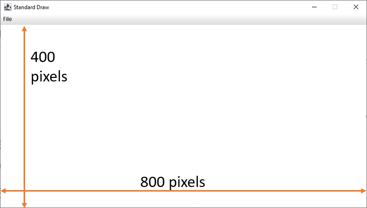
The dimension of the screen going from left-to-right (along the width) is called the x dimension. The up-and-down direction (along the height) is called the y dimension. This keeps us consistent with conventions in mathematics.
Coordinate Systems
Although it’s important to keep in mind that the canvas has dimensions expressed in pixels, PennDraw allows us to define coordinates on the screen however we’d like. By default, the coordinates of a canvas range from 0 to 1 in both the x dimension and the y dimension.
Thus, the coordinate (0, 0) refers to the bottom left position of the canvas. Coordinate (1, 1) is found at the top right of the canvas.
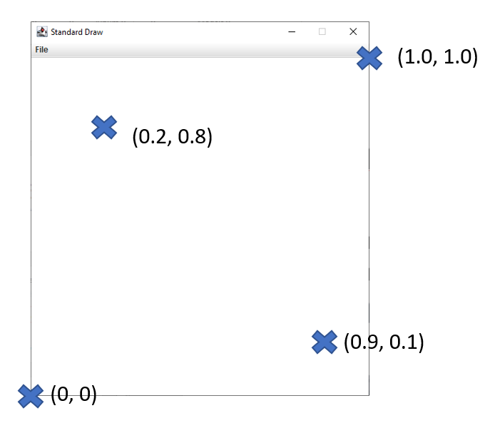
For most of the work that we do in this course, we will keep the coordinate system set in the range from 0 to 1. You should get used to referring to screen positions in this way. Here are a few important things to understand about this coordinate system:
- The "origin" is the bottom left of the canvas.
- Larger values of x coordinates refer to positions further to the right.
- Larger values of y coordinates refer to positions higher up.
- Negative coordinates or coordinates with values greater than 1 are technically valid but refer to positions not visible on the canvas.
Sometimes it also makes sense to discuss the height and width of shapes instead of just the positions of points. We can refer to these dimensions in coordinate space as well. For example, a horizontal line spanning between the left side of the canvas (x is 0.0) and the center point of the canvas (x is 0.5) would have a coordinate width of 0.5 since its width would be exactly half of the screen.
Relating Coordinates to the Canvas (Example)
First, we can set up a canvas of square dimensions, setting the width and height to the same number of pixels. Then, we can draw a rectangle with its top left vertex at (0.1, 0.8) and its bottom right vertex at (0.5, 0.6). The resulting image would look like this:

In this example, the following are true:
- The rectangle has a coordinate width of
0.4; that is, the distance in coordinate space between the right side of the rectangle at0.5and the left side of the rectangle at0.1is0.4. - The rectangle has a coordinate height of
0.2; that is, the distance in coordinate space between the top side of the rectangle at0.8and the bottom side of the rectangle at0.6is0.2.
Can you work out what the center point of the rectangle would be? If the left side of the rectangle is at x-coordinate \(0.1\) and its full width is \(0.4\), then the x-center of the rectangle would be at \(0.1 + \frac{0.4}{2} = 0.3\). If the bottom side of the rectangle is at y-coordinate \(0.6\) and its full width is \(0.2\), then the y-center of the rectangle would be at \(0.6 + \frac{0.2}{2} = 0.7\). Take a look at the image above—can you see that the center of the rectangle is at the point \((0.3, 0.7)\)?
Pen Settings
PennDraw works in a model where the programmer (you!) gives a series of instructions, one by one, to a computer that uses an abstract "pen" to draw shapes on the screen. Some instructions that you write will directly result in a new shape appearing on the screen, and others are responsible for changing how those shapes will be drawn by changing the settings of the pen. This section will explain some basics behind instructions of this second kind. For all of these instructions that change the pen settings, all future shapes will be drawn with those most recent settings until new settings are made.
Pen Radius
Whenever we ask PennDraw to draw a point, line, or group of lines on the screen, these marks will appear with a certain thickness determined by the current setting for the radius of the pen. The following image is created using PennDraw with a default radius value of 0.002, resulting in quite thin outputs:

The above image has a line, which is quite readily visible, along with a single point drawn elsewhere on the screen. Can you spot the dot, or is that a speck of dust on your screen?
If we quadruple the thickness of the pen to 0.008, the same commands to draw a line and a point result in the following:

Now that point is visible!
Pen Color
It would be boring if the only images PennDraw could generate were in black and white. Fortunately, we can change the pen settings to draw in all sorts of colors. There are two primary ways to specify a color for drawing: by name, or by RGB value.
Colors by Name
PennDraw allows you to refer to a small set of colors by a direct name. Specifically, pd.BLUE (read aloud like "PennDraw dot blue" or "pd dot blue") refers to this shade of blue:
And pd.MAGENTA looks like this:
There are a bunch of named colors that you can use:
| PennDraw Name | Color Sample | PennDraw Name | Color Sample |
|---|---|---|---|
pd.BLACK | pd.WHITE | ||
pd.RED | pd.GREEN | ||
pd.BLUE | pd.YELLOW | ||
pd.CYAN | pd.MAGENTA | ||
pd.DARK_GRAY | pd.GRAY | ||
pd.LIGHT_GRAY | pd.ORANGE | ||
pd.PINK | pd.HSS_BLUE | ||
pd.HSS_ORANGE | pd.HSS_RED | ||
pd.HSS_YELLOW | pd.TQM_NAVY | ||
pd.TQM_BLUE | pd.TQM_WHITE |
Colors by RGB Value
You're not limited to using the twenty colors to which we've given names! A color can also be specified by how much red, green, and blue is present in it. To specify a color in this way, we use three integer numbers (whole numbers) each between 0 and 255 written like (red, green, blue). For example, if we want a pure red color that looks like this, we would choose our red value to be 255 (as big as possible) and choose green and blue to both be 0.
To create this charming "twilight lavender" color, we use the RGB triple (138, 73, 107). Interpreting this triple, we see that "twilight lavender" comes from a blend of a lot of red at 138, along with a slightly smaller amount of blue at 107 and even less green at 73.
You can experiment with RGB values by clicking on the box labeled "Color" below. This is an example of a simple color picker, and you are encouraged to use it whenever you need to figure out a color's RGB code for a drawing. (You can also use a more complex one if you prefer.) As you select a new color, the red, green, and blue values update and the box also changes color.
Red Value: 204
Green Value: 204
Blue Value: 204
Using this tool, try to select each of the following colors in the color picker tool. In each case, observe the relative values of red, green, and blue.
- Black
- White
- Light Grey
- Dark Grey
- Dark Green
- Pink
- Yellow
- Teal/Cyan
- Magenta/Purple
You will pick up an intuition for the relationship between an RGB triple and its corresponding color over time. Specifying colors by RGB triples gives us fine-grained control over the colors that appear on the screen. We can make pleasing gradients by blending colors smoothly into others. For this drawing, I approximate a gradient by setting a new color, just slightly different in terms of RGB values than the previous color, before I draw each line:

Drawing Order
Just by learning about the rules of PennDraw, you probably have some idea of what drawings it’s capable of making. For example, it’s not surprising to think that we could draw a small red circle, a medium white circle, and a large blue circle all on a black background:
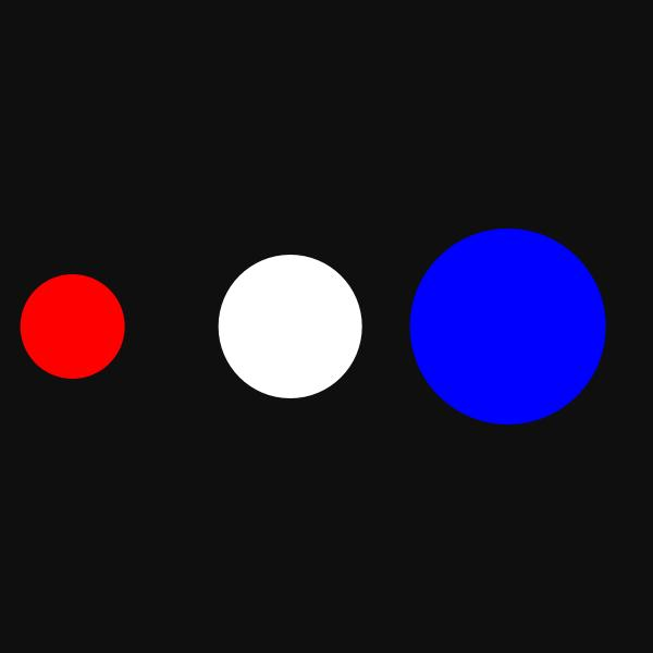
Maybe it would be interesting to draw them all as concentric circles instead, one on top of the other. Let’s see what happens when we draw the small red circle, then the white circle, and then the big blue circle:

That’s not right, it’s just the blue circle! What happened?
The issue lies in the order that I specified for drawing the circles. PennDraw draws the most recently requested shape on top of whatever else has already been drawn.
Recall that I chose to draw the small red circle first, then the white circle, and then the big blue circle. This means that the red circle and the white circle were both drawn, but they’re both hidden behind the bigger blue one.
What happens if we draw the blue circle first, then the white circle, then the red circle?

Bullseye! 😉
Running & Viewing PennDraw Programs
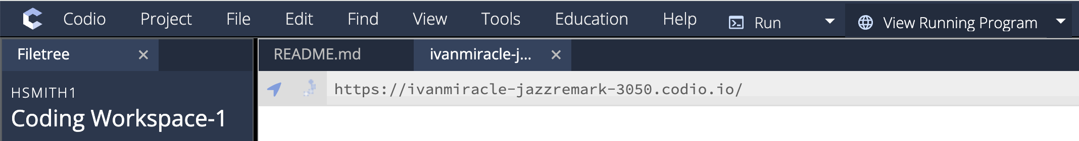
Programs using PennDraw are written in much the same way that any other Python programs would be written. There is a small difference in how we view the output of PennDraw programs compared to our first hello_world.py and hello_everybody.py programs, though. Since PennDraw draws shapes to the screen, we can't just look at the terminal to see our outputs the way that we have when observing the outputs of print statements. Instead, you will need to find the "View Running Program" button along the top menu bar in Codio and click it in order to view the drawing that your program created. In the image below, you can find that button at the top right corner.
my_house.py
For your first homework assignment, you’ll use PennDraw to create a drawing of your own. Before we get there, though, we’re going to take a guided tour through an example PennDraw illustration: my_house.py.
We’re going to build up my_house.py step by step.
A Blank Canvas on which to Paint
First, we import PennDraw and set up our canvas. Most of our PennDraw programs will start in a similar way—you always need to import PennDraw and then you'll often want to decide how big your drawing should be.
import penndraw as pd

pd.set_canvas_size(500, 500)
The first argument—meaning number—provided to set_canvas_size is the width, and the second corresponds to the height. This statement creates a blank canvas for us of size 500x500. It is important that this statement comes first so that we have the correctly sized canvas for drawing.
Our PennDraw window should look something like this now:
Beautiful Blue Sky
import penndraw as pd

pd.set_canvas_size(500, 500)

# draw a blue background
pd.clear(pd.BLUE)
Our next statement is pd.clear(pd.BLUE). pd.clear is a function that paints over the entire canvas in a single color. The color that will be used is the argument to the function, so pd.clear(pd.BLUE) fills the entire canvas with the color pd.BLUE, which, predictably, is blue. Everything else will be drawn in front of this blue background, and this will serve to be the sky in our final image.
Here is our beautiful blue sky2.

Greener Pastures
import penndraw as pd

pd.set_canvas_size(500, 500)

# draw a blue background
pd.clear(pd.BLUE)

# draw a green field
pd.set_pen_color(0, 170, 0)
pd.filled_rectangle(0.5, 0.25, 0.5, 0.25)
Our first new statement is pd.set_pen_color(0, 170, 0), which sets the color of the pen for the next shape to be drawn to be a shade of green. We use pd.set_pen_color() to change the pen color setting, and we give it three integer arguments to specify the red, the green, and the blue values of the new color. Here, we create a new color with red and blue values both 0, leaving green as the only shade blended into this color with a chosen value of 170 (between a minimum of 0 and a maximum of 255). This means that whatever we draw next will appear in this color. This statement does not draw anything to the screen, though!
The drawing comes at pd.filled_rectangle(0.5, 0.25, 0.5, 0.25). pd.filled_rectangle() does what its name suggests: draws a filled-in rectangle to the screen. The first and second arguments define the x_center and y_center of the rectangle, meaning that the center coordinate of the drawn rectangle will be at (0.5, 0.25). Interpreting these coordinates tells us that the rectangle will be centered halfway (0.5) across the screen, one quarter (0.25) of the way up.
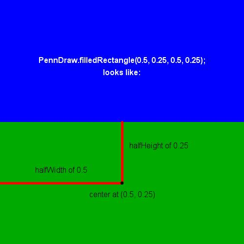
The third argument is the half_width of the rectangle, meaning the distances in coordinates between the center of the rectangle and its left and right sides. The half_width is set to 0.5 here, and since we know that the x_center of the rectangle is at x-coordinate 0.5, the rectangle will range from x-coordinate 0 on the left to 1 on the right, meaning that the rectangle should take up the full width of the screen.
The fourth argument is the half_height of the rectangle, meaning the distances in coordinates between the center of the rectangle and its top and bottom sides. The half_height is set to 0.25 here, and since we know that the y_center of the rectangle is at y-coordinate 0.25, the rectangle will range from y-coordinate 0 on the bottom to 0.5 at the top, meaning that the rectangle should take up half the height of the screen.
Here is our new green field3.

Let’s Build a Home
import penndraw as pd
pd.set_canvas_size(500, 500)
# draw a blue background
pd.clear(pd.BLUE)
# draw a green field
pd.set_pen_color(0, 170, 0)
pd.filled_rectangle(0.5, 0.25, 0.5, 0.25)
# change the pen color to a shade of yellow
pd.set_pen_color(200, 170, 0)
# draw a filled triangle (roof)
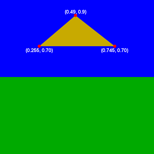
pd.filled_polygon(0.255, 0.70, 0.745, 0.70, 0.49, 0.90)
# draw the house
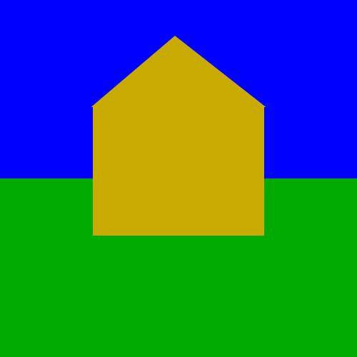
pd.filled_rectangle(0.5, 0.52, 0.24, 0.18)
We have three new statements to consider here. By now, we’re quite familiar with the first one: pd.set_pen_color(200, 170, 0). We’re changing the pen color and we’ve chosen a new color that’s a mix of plenty of red and green without any blue. The RGB triple of (200, 170, 0) is a deep gold color like this. Like always, changing the pen settings does not draw anything to the screen.
We’ll start our house by adding a triangular roof with the statement pd.filled_polygon(0.255, 0.70, 0.745, 0.70, 0.49, 0.90). pd.filled_polygon() is a tool that takes as its arguments a series of (x, y) coordinate pairs that form the vertices of the desired polygon. Specifically, the first two arguments (0.255, 0.70) represent the coordinates of the first vertex, the second pair of arguments (0.745, 0.70) mark the location of the second vertex, and finally the remaining two arguments (0.49, 0.90) mark the third vertex. These three points describe a triangle, and PennDraw will draw that triangle to the canvas. The following image marks the vertices on the triangle that we’re drawing.
We’ll finish up the structure of our house with the last new statement: pd.filled_rectangle(0.5, 0.52, 0.24, 0.18). We’ve done rectangles before, so we’ll simply state that this draws a new rectangle centered at coordinates (0.5, 0.52), just above the center of the screen, with a half_width of 0.24 and a half_height of 0.18. This gives us a rectangle slightly wider than it is tall, which has its coordinates and size chosen to match the triangle roof we already drew.
Here is our nice new home sitting on its field in front of our blue sky.
Adding a Border
import penndraw as pd

pd.set_canvas_size(500, 500)

# draw a blue background
pd.clear(pd.BLUE)

# draw a green field
pd.set_pen_color(0, 170, 0)
pd.filled_rectangle(0.5, 0.25, 0.5, 0.25)

# change the pen color to a shade of yellow
pd.set_pen_color(200, 170, 0)

# draw a filled triangle (roof)
pd.filled_polygon(0.255, 0.70, 0.745, 0.70, 0.49, 0.90)

# draw the house
pd.filled_rectangle(0.5, 0.52, 0.24, 0.18)

pd.set_pen_radius(0.005)  # thicken the pen for outline drawing
pd.set_pen_color(pd.BLACK)  # make the pen black

# draw the roof and house outlines with non-filled rectangles
pd.polygon(0.255, 0.70, 0.745, 0.70, 0.49, 0.90)  # roof
pd.rectangle(0.5, 0.52, 0.24, 0.18)  # house
It would help to have our house stand out a bit better from the background, so we’ll add a black border around the sides of the house. We start with pd.set_pen_radius(0.005), which is a statement that changes our pen thickness to be a good deal thicker. The default radius is 0.002, and our argument of 0.005 is over twice as large. This will get us a nice, pronounced border to our house.
To make sure the border is actually visible, we need to draw it in a different color from the house itself. Our next statement pd.set_pen_color(pd.BLACK) does just that. We know already that pd.set_pen_color() is used to change the pen color, and that we can give it a single color name as an argument. Now our pen is set to draw in wide black strokes.
pd.polygon() and pd.rectangle() draw the outlines of shapes described by the parameters passed to them. The space inside of the shapes will not be filled in, however.
The parameters in both cases are identical to the parameters we just gave to pd.filled_polygon() and pd.filled_rectangle() that we used to draw our house. Since we want to draw a border around those same shapes, we use the non-filled versions of those PennDraw functions to draw outlines of the exact same shapes.
Observe how
polygon()andrectangle()can be used afterfilled_polygon()andfilled_rectangle()to draw borders around shapes.
Finishing Touches
import penndraw as pd
pd.set_canvas_size(500, 500)
# draw a blue background
pd.clear(pd.BLUE)
# draw a green field
pd.set_pen_color(0, 170, 0)
pd.filled_rectangle(0.5, 0.25, 0.5, 0.25)
# change the pen color to a shade of yellow
pd.set_pen_color(200, 170, 0)
# draw a filled triangle (roof)
pd.filled_polygon(0.255, 0.70, 0.745, 0.70, 0.49, 0.90)
# draw the house
pd.filled_rectangle(0.5, 0.52, 0.24, 0.18)
pd.set_pen_radius(0.005) # thicken the pen for outline drawing
pd.set_pen_color(pd.BLACK) # make the pen black
# draw the roof, house, and door outlines with non-filled rectangles
pd.polygon(0.255, 0.70, 0.745, 0.70, 0.49, 0.90) # roof
pd.rectangle(0.5, 0.52, 0.24, 0.18) # house
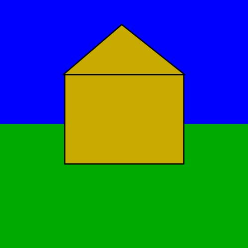
pd.rectangle(0.596, 0.44, 0.08, 0.1) # door
Let’s add a door to the house. To draw the door, we’ll need to draw its frame and then give it a doorknob.
From our previous step, our pen is already set to draw in black with a wide radius. We don’t need to change anything there, so we use pd.rectangle(.596, .44, 0.08, 0.1) to draw a small, non-filled rectangle centered at (0.596, 0.44) with halfWidth of 0.08 and halfHeight of 0.1. This is our door frame.
Our end result:

The lines of code that accomplish these two imports are: import numpy as np and import pandas as pd
Also the name of one of my favorite songs.
Not the name of any songs I know.
Code Style
Programming languages are challenging to learn. They each have a brand new syntax (an arrangement of characters, punctuation, and words) that must be adhered to in order to be properly interpreted by the computer running the program. It's important to recognize that programming languages are designed to be comprehensible to computers and people alike, and so it is considered best practice to write your programs in a way that is as straightforward and easy to read as possible.
Consider the following example of a Python program that draws a few shapes:
import penndraw as                pd
pd.filled_rectangle(0.5,.5, 0.1,  0.3)


pd.set_pen_color( pd.HSS_ORANGE )
pd.filled_circle(  0.5, .5, 0.1)
This is a functioning program, but... well, it's ugly! We have a bunch of unnecessary whitespace throughout the program: extra space between as and pd within the first line and several unnecessary lines between the calls to filled_rectangle() and set_pen_color(). Sometimes we have spaces before and after our parenthesis characters but sometimes we do not. Sometimes we have spaces after commas and sometimes we do not. Sometimes we write our number values with a leading 0 and sometimes we do not.
It's hard enough at the outset of your programming journey to create programs that run at all, so we want to avoid as much unpredictability in the presentation as possible. Observe the following code, which takes the program from above, rewrites it with consistent spacing and formatting, and adds some comments.
import penndraw as pd

#draws a background rectangle
pd.filled_rectangle(0.5, 0.5, 0.1, 0.3)

# draw an orange circle overtop the original rectangle
pd.set_pen_color(pd.HSS_ORANGE)
pd.filled_circle(0.5, 0.5, 0.1)
This program behaves in exactly the same way as its original version, but now it is formatted for consistency and clarity. The measure of a program's comprehensibility and presentation is called its style, and learning how to write programs with good style is essential for learning how to write programs at all. By following consistent style guidelines, you will be able to more quickly learn and recognize patterns of correct syntax and spot bugs when they occur. Additionally, by having your programs formatted neatly and in conventional ways, it will be easier for members of the course staff to quickly understand your code and to spot errors in the syntax. You can read the full course style guide here (TKTKTK!), although it does cover a number of features of the language that we have not yet introduced. For now, here are a few important points to follow:
- Place only one space between tokens (words, numbers, characters) when a space is required
- Limit your line length to 80 characters at the most; any longer and the line is both hard to read and to understand
- Add comments to specify the purpose of each logical block of code. It is possible to write too many comments as well as too few comments, but you should err on the side of "overcommenting" as a beginner.
- Start each file that you submit with a header comment including your name, PennKey, recitation number, example program execution, and a description of the purpose of the program.
- The example program execution is often just
python my_file_name.py, but we will see in a few chapters how program executions can vary. - The description of the program does not need to be verbose; a short explanation of what happens when the program is run is sufficient.
- The example program execution is often just
- When providing arguments to a function (e.g. specifying dimensions and positions for drawing shapes or choosing RGB values for colors in PennDraw),
- provide a single space after each comma before the next argument.
- do not add a space after the open parenthesis (
() or before the close parenthesis ()).
- Numbers between -1 and 1 should always have a leading
0provided for clarity (i.e. write0.7instead of.7)
Data Types
Learning Objectives
- To be able to define data types
- To be able to write expressions using simple data types
Overview
Computers are devices that store, retrieve, and manipulate data at extreme speeds. This simple definition really undersells the excitement of computing, of course: computers bring us interactive entertainment, they enable massive increases in human productivity, and they run the complex algorithms that form the backbone of many systems that govern our lives. They can be fun, useful, and sometimes unaccountably powerful. But, nevertheless: a computer's job is to push data around really fast.
In order for us to write computer programs, then, we need a way of understanding and organizing the data that a computer is supposed to be working with. Data types allow us to do this.
Data
Data are pieces of information. We use data to model entities & solve problems. All data in Python have a data type. Data types define the set of possible values a piece of data can have and the possible operators that can be used to manipulate values from that set of possible values in order to produce other new values as outputs.
You might be familiar with the word "operation" from grade-school mathematics, as in "order of operations" when figuring out how to evaluate an expression like 3 + 4 - (3 * 7). In that case, the operations were addition, subtraction, and multiplication, denoted by the +, -, and * operators respectively. An operator is the name that we give to the symbol that denotes the operation. In programming, operators work in a very similar way.
We'll encounter a huge variety of data types in Python, but we'll start by talking about a few simple ones to start: the int, float, bool, str, and None. These types are useful for representing numbers, text, and program logic.
Numeric Types
int is a data type that represents whole integer numeric values. These values can be positive, negative, or zero, but they must not have any fractional (decimal) parts. In Python, 3, 1, 0, -10, -1033 are all examples of int values.
Values
It would be very limiting to only have access to integer numbers, and so there is the float data type in Python that can represent numbers that also contain a fractional (decimal) part. In Python, 3.0, 1.4, 0.0, -10.10, -1033.33333 are all examples of float values. The type is called float because it's short for "floating point number", which is the official name for the way that Python represents numbers with fractional parts inside of your computer's memory.
For the most part, int and float values can be used interchangeably in Python. Sometimes it's useful for a program to expect an int specifically rather than a float; for example, we might write a program that allows a user to choose a numbered item from an entree list on a menu. In that case, it would make sense to expect that the user's answer should be an int ("I'll have the number 3, please!") instead of a float ("Could I please have the number 3.7623, extra spicy?").
Another difference between the two types is that calculations with int values will always be precisely correct. Even fairly simple calculations with float values can lead to minor amounts of imprecision due to what is effectively rounding error. The amount of error is usually so small as to be irrelevant, especially in the contexts we'll be working with in this course.
Arithmetic Operators
Recall that data types are not just defined by the kinds of information they can represent—they also describe the kinds of operators that we can use on the data that belongs to the type. For numeric types like int and float, the important operators are all mathematical. Take a look at the table below to see four commonly used operators (+, -, *, /) on the int data type. Most of them will be familiar to you already!
| Operator | Operation | Example with int values | Output Value | Output Type |
|---|---|---|---|---|
+ | Addition | 3 + 5 | 8 | int |
- | Subtraction | 4 – 6 | -2 | int |
* | Multiplication | 2 * 3 | 6 | int |
/ | Division | 3 / 2 | 1.5 | float |
Each of the four common arithmetic operators in Python follow the rules of basic arithmetic. These four operators are all examples of binary infix operators, meaning that they are placed between two values that they are operating on. These values on the left and the right of the operator are called operands.
One detail to note in the table above is that while addition, subtraction, and multiplication of two int values will always yield an int as a result, the division of two int values doesn't produce another int value. Instead, the value that is produced belongs to the float data type. This reveals an important point: the output type of an operation will not always match the types of its inputs.
Fortunately, this is a pretty minor detail. The same four operators can be used on values of the float data type—again behaving in predictable ways—and in fact the operations can be performed on int and float values mixed together.
| Operator | Operation | Example with int and float values | Output Value | Output Type |
|---|---|---|---|---|
+ | Addition | 3.1 + 5 | 8.1 | float |
- | Subtraction | 4.0 – 0.86 | 3.14 | float |
* | Multiplication | -2.0 * 3 | -6.0 | float |
/ | Division | 3.0 / 2.0 | 1.5 | float |
Note that when either the left or right operand (or both) are float values, then the output type is always float.
Modulo & Integer Division
There are two additional operators for numeric types that are slightly more complicated than the common arithmetic ones. These are the % ("modulo" or "mod") operator and the // ("integer division") operator. Both of these are again defined for int and float, but we'll generally stick to using them with int values.
The integer division operation allows us to divide two int values and get an int as a result. The way that you can think about how this works is that we do regular division arithmetic, and then truncate the result by removing the fractional part (the part after the decimal). Whereas 3 / 2 (regular division) is 1.5, 3 // 2 (integer division) is 1. Generally speaking, if we write a // b, then we're calculating the number of times that b "goes into" a. Check out some of the examples in the table below.
| Example Expression | Example Result |
|---|---|
16 // 5 | 3 |
15 // 5 | 3 |
14 // 5 | 2 |
3 // 7 | 0 |
-11 // 2 | -5 |
Modulo (or "mod", for short) is an operation that complements integer division. When we write the expression a % b (read aloud like "a mod b"), we are calculating the remainder left after dividing a by b. For example, we might write 16 % 5 in order to evaluate the remainder after using integer division to divide 16 by 5. We find that 5 "goes into" 16 3 times, making 15. Thus, the remainder after dividing 16 by 5 is equivalent to 16 - 15, or 1. Sometimes this is easier to learn by example, so here are a couple of tables with plenty of examples. In the first, we see what happens as we change the number on the lefthand side.
| Example Expression | Example Result |
|---|---|
0 % 3 | 0 |
1 % 3 | 1 |
2 % 3 | 2 |
3 % 3 | 0 |
4 % 3 | 1 |
5 % 3 | 2 |
6 % 3 | 0 |
The output of a % b is always a number between 0 and b - 1. Moreover, as we increment a one by one, we see that the output increases by one each time until it wraps back around to 0 and starts the pattern again.
Now, let's look at what happens when we fix the lefthand value and "mod it" by a bunch of other different numbers:
| Example Expression | Example Result |
|---|---|
12 % 1 | 0 |
12 % 2 | 0 |
12 % 3 | 0 |
12 % 4 | 0 |
12 % 5 | 2 |
12 % 6 | 0 |
12 % 7 | 5 |
12 % 13 | 12 |
If a is evenly divisible by b, then a % b will always output 0. If a is less than b, a % b will always output a. Can you think about why this two facts are true?
Example: Pizza Party
Suppose I'm having a pizza dinner with my friends. If I have thirteen pizzas with eight slices and there are fifteen of us, what is the minimum number of full slices we can all expect to eat if we share evenly? To calculate the result, we can first think about how to write the expression that calculates how many slices of pizza we have in total.
13 * 8 # eight slices per pizza, thirteen pizzas
Next, we want to figure out how many full slices per person we'll have if we share evenly. We could try to calculate this with regular division to determine the result. The expression that does this is (13 * 8) / 15. (Technically the parentheses are optional, but I recommend using them liberally throughout your programs to make sure that your order of operations is always what you're expecting.)
print("Calculating number of slices per person...")
print((13 * 8) / 15)
If we run this program, the output is 6.933333333333334. This answer is mathematically accurate, but it doesn't answer the question as asked. We want to know the number of full slices per person—I don't know about you, but I don't know how to cut a pizza slice into .933333333333334ths.
Switching the expression to use integer division (//) should solve the problem:
print("Calculating number of full slices per person...")
print((13 * 8) // 15)
Looks like each person will get 6 slices of pizza. But we know from our first attempt that every person could actually have a few more bites of pizza each. If we divvy out 6 slices of pizza per person, there will be some slices left over. How many? This is something that we can answer with the % operator! What we want is to know the remainder after dividing 13 * 8 slices of pizza over 15 people, so we write the program like so:
print("Calculating number of slices remaining...")
print((13 * 8) % 15)
We have fourteen slices left over, it seems. We can check our work to verify that this makes sense: 13 * 8 is 104. 15 goes into 104 6 times, and 15 * 6 equals 90. After all 15 people get their 6 slices each, there will be 104 - 90, or 14 slices remaining.
Booleans
Types aren't just about numbers! We can have data types containing values that represent other entities, like truth and falsehood. The bool data type consists of just two values: True and False. That's it—just those two! They're spelled exactly that way (note the capital T and F) and they don't take quotes around them like we saw for printed text earlier. bool is short for "boolean", which is the name of the system of logic using only these two possible values.
Logical Operators
The bool data type comes with a few important operators that represent logic concepts of conjunction, disjunction, and negation; or, more simply, the concepts of "and", "or", and "not", respectively. The operators are spelled out as words in this case, unlike the ones that we used for arithmetic. That is, the operator for "logical and" is literally just: and. or and not round out the trio, and they work by combining boolean values based on the following rules encoded as truth tables below.
a | b | a and b |
|---|---|---|
True | True | True |
True | False | False |
False | True | False |
False | False | False |
To summarize: and is an operator that evaluates to True only when the left and right operands are both True. Otherwise, it evaluates to False.
a | b | a or b |
|---|---|---|
True | True | True |
True | False | True |
False | True | True |
False | False | False |
To summarize: or is an operator that evaluates to True when at least one of the left or the right operands are True. Otherwise, if both are False, it evaluates to False.
a | not a |
|---|---|
True | False |
False | True |
not is an example of a unary operator, meaning that it operates on only a single value.
Similar to operators on numeric values, logical operators can be chained together to create longer expressions. These expressions are generally evaluated left-to-right with the official order of operations setting not operations to be evaluated first, followed by and, then by or. This can be a bit confusing to remember, so you are again encouraged to use parentheses liberally in order to enforce your desired order of operations.
Simplifying bool Expressions
Let's take a look at a quick example, evaluating not (True and False) or not True and not False, where on each line we write a new, simplified expression.
not (True and False) or not True and not False
# start by evaluating not (True and False), which
# means we need to first solve the contents of the parentheses.
not (False) or not True and not False
# not (False) is just True
True or not True and not False
# in order to handle the or, we have to simplify its right side
True or False and not False
True or False and True
True or False # from definition of "and"
True # from definition of "or"
Therefore, the expression not (True and False) or not True and not False has the value of True. We can verify that by printing it out:
print(not (True and False) or not True and not False)
Strings
In our very first code example for this course, we had our program print out the message Hello, World!. In order to do so, we specified the message as text placed within a pair of quotation marks. Text values like this belong to the data type named str (short for "string"). Any sequence of characters (individual letters, numbers, punctuation, or spacing like spacebar or tab) placed within a pair of quotation marks can be a str value. There is no limit to the number of characters that can be contained in a str value.
Here are several examples of str values:
"Hello, World!""Harry S. Smith""3330 Walnut Street""!@#$%^&*()0123456789"
When we write out strings in our programs, we can actually enclose them within pairs of single quotes ('), double quotes ("), or triples of single or double quotes (''' or """). This can come in handy when the text you want to represent has one or both of these quote characters within it.
Here are a few more examples of str values, showing off the different quote styles:
'This is a valid str.'"This isn't a valid str.""""This is a str with triple "s..."""'''This is a str with triple 's...'''"""This isn't "easy" to read, but it is a valid str."""
Strings are sequences of characters, and it often makes sense to discuss the size or length of a str value. In Python, the length of a str is the number of characters it contains. This includes all characters: letters, numerals, punctuation, spaces. Here is a table of examples, including the lengths of each str value.
str | Length |
|---|---|
| "Harry" | 5 |
| "HarrySmith" | 10 |
| "Harry Smith" | 11 (the space counts!) |
| "1100?" | 5 (digits & punctuation count, too ) |
| "👀" | 1 (str values can contain emojis, which are each one character) |
| " " | 1 (non-empty because it contains a space bar) |
| "" | 0 (an empty sequence of characters is still a valid str) |
That last str there—""—is called the "empty string." It's a valid string, and it is a sequence of zero characters.
Operators for str
There are lots of different ways to manipulate strings in Python, but we'll start by introducing just two simple operators. The first defines the concatenation operation, which is the process of joining two strings together end-to-end. The operator itself will look very familiar: +!
In order to create the string "CIS1100", we could concatenate the strings "CIS" and "1100" together like so:
"CIS" + "1100"
In order to see the result, we can print it out:
print("CIS" + "1100") # prints CIS1100
There are a few important things to pay attention to here. The first is that there is no space added when concatenating two str values: "CIS" + "1100" takes all three of the characters of the first string and then all four of the characters of the second string with nothing added in between, so the resulting "CIS1100" has exactly seven characters. This means that if we concatenate two strings that represent words or names, the result will look a little clumsy:
print("Grace" + "Hopper") # prints GraceHopper
In order to put a space between them, we need to add that space as a character to one of the strings.
# both examples print out Grace Hopper
print("Grace " + "Hopper")
print("Grace" + " Hopper")
The second important thing to note about the expression "CIS" + "1100" is that its second string is, in fact, a str value, and not an int value! Even though the contents of the string are the characters 1, 1, 0, 0 and are therefore all numerals, the fact that they are contained within a pair of quotes means that they are interpreted as components of a str value. The importance of this is emphasized by the fact that you cannot concatenate a str with a value of another data type in Python. Trying to execute the following line of code will result in an error, including the message "can only concatenate str (not "int") to str".
print("CIS" + 1100)
This means that if you do "1" + "1", you won't get 2, because both 1's are strings:
print("1" + "1") # prints 11
Our second str operation will be string repetition using the * operator. In this case, we can provide a str value on the left hand side of the operator and an int value on the right hand side of the operator. This number on the right tells us how many times to repeat the text on the left. For example, we could write some lines of code that let your friends know how funny they are:
print("ha" * 1)  # ha
print("ha" * 2)  # haha
print("ha" * 4)  # hahahaha
print("ha" * 10) # hahahahahahahahahaha
Or, you could imitate a villain from a horror movie:
# I won't share the output here, but try to run this line.
print("All work and no play makes Jack a dull boy." * 1000)
None
This is a special type that contains only a single value: None! From the Python documentation:
It is used to signify the absence of a value in many situations.
Sometimes we may ask the computer to perform some operation for which there is no result, in which case we might get the answer of None in return. There are no operators that can apply to None. We will not use None much in the beginning of the course, but you should be aware of it as it begins to crop up in later lessons.
Relational Operators
There is a group of operators that can be applied to values of different data types, and so we'll conclude our discussion of data types with these, called relational operators. These operators provide us ways of comparing two values for order or equality. The output data type is always a bool.
Equality (== and !=)
The == operator, called "double equals" when read aloud, allows us to ask if two values are equivalent to each other. This operator works with values of any different types. The following table shows a few examples of its usage:
| Expression | Result |
|---|---|
4 == 4 | True |
5 == 4 | False |
4.0 == 4 | True |
"4" == 4 | False |
"4" == "4" | True |
"4" == "4.0" | False |
"Comp" == "Sci" | False |
"Comp" == "Comp" | True |
True == False | False |
(4 + 3) % 6 == 3 // 2 | True1 |
(4 + 3) is 7. 7 % 6 is 1. On the right hand side, 3 // 2 is 1 since we're using integer division. So, the expression simplifies to 1 == 1, which is True.
Numbers (int and float values) are compared based on their numeric value, and so 4 and 4.0 are considered equal. str values are compared character-by-character, so "4" and "4.0" are not equal: their first characters are the same, but they differ after that point. The last row of the table demonstrates that we can compare the results of entire expressions.
We also have the != ("not equals") operator available. It allows us to ask whether two values are different, and it produces exactly the opposite result compared to using ==. The following table uses the same expressions as the previous table, but replaces != with ==.
| Expression | Result |
|---|---|
4 != 4 | False |
5 != 4 | True |
4.0 != 4 | False |
"4" != 4 | True |
"4" != "4" | False |
"4" != "4.0" | True |
"Comp" != "Sci" | True |
"Comp" != "Comp" | False |
True != False | True |
(4 + 3) % 6 != 3 // 2 | False |
The inclusion of the None type in Python means that sometimes we need to ask the question: "does this value exist?" We do so by comparing the result to None, e.g. "yes" * 2 == None or 4.0 - 3.9999999 == None. In both cases, and indeed most of the time, the answer is False.
Ordering (<, <=, >, >=)
Sometimes, we may be interested in determining how two values compare to each other: is this less than that? is this number greater than or equal to this other one? These next four operators (<, <=, >, >=) allow us to do these comparisons in Python. Like the equality operators, these operators both produce bool values as the output type; however, the comparison operators must take in two values of the same type. Values should be both numeric [int or float], both str, or both bool on the left and the right hand side. When you compare two strings with these operators, they are compared lexographically. The next table has some examples.
| Expression | Result |
|---|---|
4 < 5 | True |
4 > 5 | False |
9 <= 9 | True |
9 < 9 | False |
"apple" < "banana" | True |
"carrot" > "banana" | True |
"banana" > "banana" | False |
True > False | True |
100 / 12 <= 4.5 * 2 | True |
4 > "howdy" | 🚨Error! Type mismatch. 🚨 |
True <= None | 🚨Error! Type mismatch. 🚨 |
Python also allows us to chain these ordering operators together. This is a convenient and succinct way of determining whether or not a value fits within a certain range. For example, 0 < 10 < 20 evaluates to True because 0 is less than 10 and 10 is less than 20. We can also chain str values in the same way, and so "zebra" > "panda" > "elephant" is another True statement since "panda" comes lexicographically before "zebra" but after "elephant". When we write one of these expressions, Python evaluates them as a series of individual binary comparisons strung together with and operators. We could write 10 >= 0 > -10 as 10 >= 0 and 0 > -10, which is in fact how we would have to express this in many other programming languages. We can get a bit creative with the ordering of these chained operators, although it can be a bit confusing to break down and understand. The following boolean expressions all have equivalent values:
| Expression |
|---|
5 < 10 > 8 |
5 < 10 and 10 > 8 |
True and 10 > 8 |
True and True |
True |
Example: Leap Years
Let's use our newfound knowledge of these arithmetic, relational, and logical operators to write a program. We'll write code that determines whether or not a year counts as a Leap Year. From Wikipedia:
A leap year [...] is a calendar year that contains an additional day [...] compared to a common year. The 366th day [...] is added to keep the calendar year synchronised with the astronomical year or seasonal year.
Generally speaking, every four years, we have an additional day in the calendar: February 29th, my half-birthday. But this is actually an oversimplification, since we skip the Leap Year every 100 years in order to be properly aligned. But! That would be too few Leap Years, so we reinstitute the Leap Year every 400 years even though we'd normally skip it due to the 100-year-rule. In short, a year is a Leap Year if:
- The year number is divisible by four and the year number is not divisible by 100, or
- The year number is divisible by 400
In order to write a program that can do this calculation, we'll need a way of determining if a number is divisible by another. Recall that the % (modulo) operator has the property that if a is divisible by b, then a % b will be 0. So, we have the ability to write a few divisibility tests by modding the year and comparing the result to 0.
- To determine if a year, e.g.
2024, is divisible by four, we write2024 % 4 == 0. - To determine if a year, e.g.
2024, is not divisible by100, we write2024 % 100 != 0. (Note the use of!=instead of==.) - To determine if a year, e.g.
2024, is divisible by400, we write2024 % 400 == 0.
We've now come up with a way to write three "questions" about the year whose answers will be True or False depending on the divisibility of the year. We still need some way of connecting these three questions into the larger one about Leap Years. We'll combine these smaller questions using logical operators—and & or—based on our definition of a leap year. Recall the definition I wrote above:
A year is a Leap Year if the year number is divisible by four and the year number is not divisible by 100, or the year number is divisible by 400
Notice that the definition above already includes the words and & or, giving us a pretty strong hint about how to solve the problem! If we replace each of the subquestions about divisibility with the expressions that we came up with to test them, then the program starts to take shape:
A year is a Leap Year if (the year
% 4 == 0andthe year% 100 != 0)or(the year% 400 == 0)
If we replace "year" with a year number that we want to test, we can write a program that gives us an answer to the Leap Year question:
print("Is 2024 a leap year?")
print(((2024 % 4 == 0) and (2024 % 100 != 0)) or (2024 % 400 == 0))
This program prints True, which is correct, since 2024 is a Leap Year. Happy half-birthday to me!
To test it on different years, we have to change each instance of the year in the expressions to represent that new year. This can be a little tedious, but we'll see a better way of doing this in the next section. Below is an example of extending the Leap Year program to test three different years. Can you predict what the program should print? When you run it, does it match your expectations?
print("Is 2024 a leap year?")
print(((2024 % 4 == 0) and (2024 % 100 != 0)) or (2024 % 400 == 0))

print("Is 2025 a leap year?")
print(((2025 % 4 == 0) and (2025 % 100 != 0)) or (2025 % 400 == 0))

print("Is 2000 a leap year?")
print(((2000 % 4 == 0) and (2000 % 100 != 0)) or (2000 % 400 == 0))
Variables
Learning Objectives
- To know what a variable is
- To be able to declare variables
- To be able to solve problems using expressions of variables & data values
Overview
Now that we have a good understanding of data types, we have a picture of some of the kinds of information that a computer can represent and manipulate. As we saw in leap_year.py, however, even simple questions can be unwieldy when we have to answer them with long expressions written in a single line. We will now introduce variables, which allow us to organize the information in our program by giving names to pieces of data.
Variables
A variable is a named portion of computer memory used to store a data value. In this way, a variable is like a box with a name. The box can store any kind of data within it, but it only ever stores one piece of data at a time. The box is given a name, like a label pasted to the front, and placed on a shelf. Whenever we want to use the data stored in the variable, we refer to it by name. This is like searching for the box with the matching label on our shelf and pulling out whatever is contained inside.
Variables, as the name suggests, are allowed to vary overtime. Their contents can be written and overwritten as many times as we like. To continue the analogy, we're allowed to replace the contents of our boxes with something new whenever we need: we simply find the box by name, remove its previous contents, and add something new instead.
Variables allow us to have the computer "remember" data between different lines of our program. We can do our computation in stages now, writing an expression to calculate an intermediate result and then saving that result inside of a variable for later use.
To summarize:
- Variables are portions of computer memory that always store a data value.
- Variables have names, which allow us to refer to them throughout a program.
- Variables can have their contents updated throughout a program.
Declaring Variables
In order to use a variable in Python, it must first be declared. Variable declaration is the process of creating a variable by giving it a name and an initial value. This is pretty simple to do in Python:
year = 2024
In this example, we declare a variable called year. It contains the int value 2024. The general pattern for variable declaration is new_variable_name = <expression> where the left-hand side contains any valid identifier and the right-hand side consists of any expression, the resulting value of which will be stored inside of the variable.
Between the name and the initial value of the expression, we have a single equals sign (=). This is called the assignment operator, and it should be read as a assertive statement rather than a question. When you write the following line, you are putting on your royal crown and waving your golden scepter around, proclaiming, insisting, demanding that the variable called first_name shall absolutely, decisively, incontrovertibly store the value "Harry" until further notice.
first_name = "Harry"
I am being dramatic here for emphasis about something that is often confusing. In algebra, the equals sign is often used as part of a question: "what value or values of x make the left- and right-hand sides equal?" That is not what is happening here! We are putting a value in a box, not asking about truth values (that would be done with ==) or solving equations.
Naming Conventions
In Python, we use snake_case to name our variables. Variables should consist only of lowercase letters, underscores (_), and digits. Variables should start with a lowercase letter. In order to break up variable names that consist of multiple words, we separate those words with underscores. Variable names should be chosen to be descriptive. There is a tension between being descriptive and being verbose, but editor tools like autocomplete make it easier to stomach longer variable names by preventing you from having to type them out completely. Let's look at a few more variable declarations and observe the style used:
| Declaration | Comment |
|---|---|
score = 99.9 | valid |
last_name = "Smith" | valid |
is_mouse_pressed = False | valid |
isMousePressed = False | invalid — use _ to separate words |
avg_pt_ht = 180 | technically valid, but the use abbreviations make it very hard to read! |
avg_patient_height = 180 | a better compromise for the row above |
color_2 = "red" | valid, although ugly to the author's eye 🤷 |
Using Variables
Once a variable has been brought into existence by declaring it, we can use its value inside of other expressions. In this first example, we declare the variable three, put the int 3 inside it, and then immediately print out its value.
three = 3
print(three) # prints out 3
We can use variables as part of other expressions. Here, we calculate the value of \(1.6^2\) by multiplying x with itself:
x = 1.6
print(x * x) # prints out 2.5600000000000005 due to some rounding error.
Indeed, we can even declare variables in terms of other variables!
a = 10
b = 20
c = a + b
print(c) # prints out 30
It's important to note that the value stored inside of a variable during declaration and assignment is the result of evaluating the right-hand side expression at the moment the assignment is done. That means that on the third line of the previous snippet, we calculate the value of a + b based on the values stored inside of a and b—10 and 20—at that time, and then store the result (30) inside of c. If we later changed the values of a or b, the value of c would not be changed as a result. Only an assignment to c can change the value of c.1
Reassigning Variables
As referenced above, it is possible to change the value stored inside of a variable. The syntax for doing so is actually identical to the syntax for declaring a variable, since in Python we declare a variable by assigning a value to it.
coin = "heads"
print(coin) # prints heads
coin = "tails"
print(coin) # prints tails
Updating a variable lets us do things like keep count of how many times an event has occurred or change a person's personal details in a dataset. A general rule of thumb that you will want to keep in mind, though, is that it's not a good idea to change the type of information that a variable stores over time. This makes it hard to keep track of what you can and can't do with a variable throughout your program, and it means that probably the name of the variable no longer describes its contents.
my_name = "Harry Smith"
print("My name is:")
print(my_name)
my_name = 27
print("In three years, I will be:")
print(my_name + 3)
The above program runs, although it is quite confusing. If you were to write this code and then come back to it a few days late, you might find yourself asking: "Why is my_name 27? Shouldn't a name be a string?" You should always make an effort to preserve the type of a variable over time.
Before we move on from updating variables, let's take a look at one last example.
count = 0
count = count + 1
count = count + 2
count = count + 10
print(count) # What gets printed?
At a first glance, this might be quite confusing! How do we reassign a variable in terms of itself? The answer comes by following the rule described above: the value stored inside of a variable during assignment is the result of evaluating the right-hand side expression at the moment the assignment is done. On the first line, count is set to be 0. When the second line is executed, we first evaluate the right-hand side. At this moment, count has the value 0 stored inside, so the value of count + 1 is 1. We store the value 1 inside of the variable on the left-hand side, which is count. After line 2, count now has the value 1. We repeat the process on line 3: count is currently 1, so we compute the value 3 on the right-hand side and store that inside of count, the variable on the left. Repeat once more, where the value of the expression on the right is 13--can you see why?--and so when we get to line 5, count is finally storing the value of 13, which is what gets printed. Verify this for yourself by running the program.
Reassigning a variable in terms of itself is a common practice. It allows us to count the number of times certain events happen, or to accumulate interest by repeatedly multiplying a quantity by an interest rate, or to run a timer counting down to zero with each passing second.
Leap Year, Redux
Let's use what we know about variables to improve our leap_year.py program. We want to make it easier to read, and we want to make it so that we can easily adapt it to test different years without having to change the year number in several different places. To refresh your memory, here is where we left off with leap_year.py:
print("Is 2024 a leap year?")
print(((2024 % 4 == 0) and (2024 % 100 != 0)) or (2024 % 400 == 0))

print("Is 2025 a leap year?")
print(((2025 % 4 == 0) and (2025 % 100 != 0)) or (2025 % 400 == 0))

print("Is 2000 a leap year?")
print(((2000 % 4 == 0) and (2000 % 100 != 0)) or (2000 % 400 == 0))
In order to calculate whether a year is a leap year, we needed to do three divisibility checks on the year number. This means that any time we want to test whether a different year is a leap year, we have to remember to change three different numbers in the same line. This is a bit tedious, and can be remedied by declaring a variable to store the year that we're testing.
year = 2024
print(((year % 4 == 0) and (year % 100 != 0)) or (year % 400 == 0))
Now, if we want to test the year 2023 or 1900 or 200 or 2000, all we need to do is change the value stored inside of the variable year and that updated value will be used in the calculation.
In this case, we are still fitting all three divisibility checks on the same line. In my opinion, this makes the line very hard to read and understand: it's too long, and there are too many different numbers presented without explanation. Instead, we could take each of the divisibility tests and write them as their own individual boolean expressions, saving the result of each in its own variable with a descriptive name:
divisible_by_4 = year % 4 == 0
divisible_by_100 = year % 100 == 0
divisible_by_400 = year % 400 == 0
Finally, we can rewrite the full test in terms of the new variables that we've declared:
is_leap_year = (divisible_by_4 and not divisible_by_100) or divisible_by_400
Thanks to our descriptive variable naming scheme, the full leap year calculation is now written in code in almost exactly the same way we would describe it in plain, natural English. Putting all of this together and adding print statements, we now have the following program:
year = 2024
print(year)
print("Calculating if above year is a leap year...")

divisible_by_4 = year % 4 == 0
divisible_by_100 = year % 100 == 0
divisible_by_400 = year % 400 == 0
is_leap_year = (divisible_by_4 and not divisible_by_100) or divisible_by_400
print(is_leap_year)
We have spread the program over more lines, but each individual line is now a bit easier to understand. We have generated a program that is self-commenting, meaning that it is written in a way that makes the purpose of the code clear without much additional explanation required. This is one of the benefits of Python as a language and it is something that we should strive for in the programs that we write throughout this course.
More Powerful Printing 🖨️
As you've seen in the examples throughout this chapter, it's possible to use print() to view the contents of a variable. Want to know what a variable stores at some point in your program? Print it out!
mystery = "hooooo egassem terces"[::-1]
print(mystery)
Now that we are capable of writing programs that manipulate data, it will be helpful to have concise but informative ways of printing out one or more values. To start, if you want to print out multiple pieces of information on a single line, each separated with a space, you can do so by interleaving commas (,) between the things you want to print.
num_bottles = 99
print(num_bottles, "bottles of beer on the wall,", num_bottles, "bottles of beer...")
# prints out "99 bottles of beer on the wall, 99 bottles of beer..."
This is a nice, straightforward way of putting a bunch of different pieces of information on the same output line. Notice that while variables have their values printed, the strings that we put in (recognize them by the " characters that surround them) are printed literally. Nowhere in the printed output do we see the literal n, u, m, _... characters of num_bottles: the name of the variable is not printed.
Each time we write print(), the information inside of that print statement all goes on its own line. Modifying the previous program slightly, we see that the extended output is now spread across multiple lines:
num_bottles = 99
print(num_bottles, "bottles of beer on the wall,", num_bottles, "bottles of beer...")
print("Take one down, pass it around!")
num_bottles = num_bottles - 1 # decrease the value stored in num_bottles by one
print(num_bottles, "bottles of beer on the wall.")
99 bottles of beer on the wall, 99 bottles of beer...
Take one down, pass it around!
98 bottles of beer on the wall.
We can take this a step further using f-strings. An f-string is a slight variation of a typical string that is denoted by placing an f right before the start of the string, as in:
msg = f"this is a simple f-string. You can tell by the f."
If we printed out msg, the output would be exactly the content of the f-string seen in the example above; that is, on their own, f-strings behave exactly like other strings. The interesting extension that f-strings provide, however, is that we can leave slots inside of the f-string to be filled with the result of an expression. The slots are denoted with curly braces ({}) and they can be filled with any expression that you want to write.
age = 27
birthday = "August 29"
print(f"I'm {age}, and after {birthday}, I'll turn {age + 1}.")
If we run this program, we'll see the following message printed:
I'm 27, and after August 29, I'll turn 28.
How do we get that result? Notice that any characters outside of the curly brace pairs are printed literally (i.e. "I'm", ", and after ", ", I'll turn ", "."). The stuff inside of the braces is treated as a normal Python expression that is not part of a string. The values of these expressions can be determined based on the variables that have been declared and assigned previously. So, the first slot is filled with the value of the expression age, which is 27. The second is filled with the value of the expression birthday, which is "August 29". Finally, the third is filled with age + 1, which has the value of 28. These f-strings can take some getting used to, but they are just about the most concise way to pack a bunch of information into a single line of text. The equivalent way of doing this with commas in the print statement looks like this:
print("I'm ", age, ", and after ", birthday, ", I'll turn ", age + 1, ".")
It's not so different, but there's a bit of fussiness involved in keeping track of all the quote pairs and commas. I recommend that you practice using f-strings.
This is only true for some data types in Python. Before long we will see examples where this does not hold when dealing with list or dict values.
Conditionals
Learning Objectives
- Create and evaluate boolean expressions that answer questions about the state of a program's data
- Use
if,elifandelsekeywords to build conditional statements that control the flow of a program - Choose among several enumerated possibilities using the
match&casekeywords
Overview
"You ever made a decision?"
"No, I never did that." -- Joan Didion, Play It as It Lays
Earlier on, we introduced the concept of control flow in a program as the order in which its lines of code are executed. Our first programs used only the default control flow, wherein lines are executed from top to bottom and only time each. This was sufficient for simple calculations, printing, and programs that made static drawings, but it does not allow for our programs to make any decisions. In this chapter, we will apply our knowledge of boolean expressions and introduce new control structures in order to write programs that are capable of making choices based on information available to them.
Conditions & Conditionals
In order to write programs that respond to different situations, we'll need to introduce the concepts of conditions and conditionals. Conditions are defined as the states of the data in your program. A program's data can include things like values stored inside of variables, information requested from outside sources like the internet, or user input like mouse clicks and button presses. Conditions are defined using boolean expressions, or expressions of values and variables that evaluate to a boolean type. You can refer to the chapter on data types for a refresher on the bool type and expressions that produce boolean values.
Conditionals are the structures that we use to make decisions based on the conditions that we define. These decisions take the form of questions like: "which of these actions should I take?" or "should I choose to do this next step?"
An example of a condition that you would be aware of as a pedestrian in Philadelphia is whether or not the light facing you at an intersection is currently green. This condition could be true or false—the light might be green, or it might currently be yellow or red instead. The conditional that you use in your "walking program" is that if the condition is met; that is, if the light is green, then you will cross the intersection. If that condition is not met and the light is not green, then you will wait.
Conditions as Boolean Expressions
Recall that boolean expressions are expressions that evaluate to bool values, i.e. either True or False. Our first boolean expressions were fairly straightforward and had consistent and predictable results.
3 > 4 and 9 == (81 / 9)                     # always True
not True and True or False and not False    # always False
Now that we are familiar with the concept of variables, we are able to write boolean expressions that will produce different results based on the values stored within those variables. For example, without context, it's impossible to evaluate whether the following expression is True or False:
x % 3 == 2 and x > 5
x, as a variable, could store any number at all. The result of this expression depends on the value that we've placed in that box. Can you think of a value of x that would cause the expression to evaluate to True? What about False?
# What values of x would make this program output True?
# What about False?
x = ??? # Change this line and run the program to experiment.
print(x % 3 == 2 and x > 5)
When we use variables as part of boolean expressions, we are able to test conditions about the state of the world that our program represents. We build these boolean expressions by comparing values with relational operators and combining other boolean expressions together with logical operators.
Worked Examples of Writing Expressions to Test Conditions
"Is the number of tickets sold equal to the capacity for the venue?" or "Is the user's password long enough to be valid and is it different from their username?" are the kinds of useful questions that we can formalize as boolean expressions with variables: sometimes the answers will be "yes" and sometimes "no", all depending on the values stored in the underlying variables.
print("Is the number of tickets sold equal to the capacity for the venue?")
print(num_tickets == venue_capacity)

print("Is the user's password long enough to be valid and is it different from their username?")
print(len(password) >= 8 and password != username)
To determine if a password is long enough, we compare the length of the password (len(password)) to a fixed minimum length of 8 using the >= operator. To check to see if a user's password and username are different, we use the != ("not-equals") operator to compare them. In order to combine these two smaller boolean expressions into a large one that models our condition, we join the two using the logical and: the condition of whether or not a password is acceptable is met if and only if the password is both long enough and distinct from the user's username.
One-Way Streets in Center City
In Center City Philadelphia, a numbered street is one-way heading South if its number is even and its number is not 14.1 Try practicing the process of modeling conditions by writing a boolean expression that whether or not a street is one-way heading South: "Is the given street number even and is its number not 14?"
To answer this question, we'd need to know the street number. It's not specified in the question, which means that we'll think of it like a variable: street_number seems like a suitable name.
Next, we need to know how to test whether or not a street number is even to build the first part of the boolean expression. A number is considered even if it is divisible by two, and we can test divisibility using the modulo (%) operator: street_number % 2 == 0 is an expression that evaluates to True when street_number is even.
Then, we have to be able to test if our street number is not 14. Like we did in the password example, we can use the != operator to have a comparison evaluate to True when the two values being compared are different. street_number != 14 evaluates to True when street_number does not store the value 14.
Finally, we can build our full condition by combining these smaller boolean expressions together with a logical operator. We want the condition to be True only when both sub-expressions are True; that is, when the street number is even and the street number is not 14. This will be a good use of the and operator.
street_number = 2 # Change this line and run the program to experiment.
print(f"Does {street_number} Street run one-way south in Center City Philadelphia?")
print(street_number % 2 == 0 and street_number != 14)
"14th Street" doesn't actually exist in Philadelphia: we call it Broad Street instead. Furthermore, Broad Street is a two-way street instead of a one-way.
Conditionals: if, elif, and else
Conditionals allow us to control the flow of a program based on conditions defined using the values in the program. Conditionals are defined in Python using three special keywords: if, elif, and else. We will start by introducing the if statement.
The if Statement
"
ifmusic be the food of love, play on." — William Shakespeare
Whereas before we executed all lines of code in the program from top to bottom, our first conditional—the if statement—will allow us to specify a portions of our program that should be run only if a certain corresponding conditions are met. We can understand the behavior of if statements by examining the flow chart below:
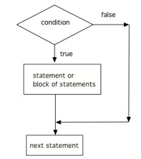
On reaching the if statement, we test a condition. If that condition is True, then we execute the corresponding statement or block of statements. If the condition is False, then we skip over all corresponding statements and resume program execution at the first line of code following the skipped statements. The motto to remember when you see a single if statement is: "I am now choosing whether or not to do something."
The if statement is built using the if keyword, a boolean expression followed by a colon (:) and a body of statements indented one level further than the line with the if. The structure for such a statement looks like this:
if my_boolean_expression:
	statement_one
	statement_two
	...
	statement_last
For example, perhaps we want to write a program that helps us determine whether or not a variable num is divisible by 5. We can start by assigning num = 10 and observing the result.
num = 10
print("Printing a message if {num} is divisible by 5...")
if num % 5 == 0:	# if, followed by our boolean expression defining the condition
	print("Yes!")	# the statement to be executed if condition is met
When the program is run, we get the following output:
Printing a message if 10 is divisible by 5...
Yes!
Success! Since 10 is divisible by 5, our boolean expression num % 5 == 0 evaluates to True: our condition is met. So, we evaluate the statements in the indented block following the line with if. In this case, that is a single line: print("Yes!"). Our output consists of two printed lines.
We could change the value of num, thereby changing the state of our program, and observe the result.
num = 11	# Trying again but changing 10 --> 11
print("Printing a message if {num} is divisible by 5...")
if num % 5 == 0:	# if, followed by our boolean expression defining the condition
	print("Yes!")	# the statement to be executed if condition is met
When the program is run, we get the following output:
Printing a message if 10 is divisible by 5...
Only one line is printed! The condition is not met—num % 5 == 0 evaluates to False this time—and so we skip all statements in the indented block. Remember: with an individual if, you are choosing whether or not to do something.
The indented blocks that you find underneath each of the if statements define the lines of code that will only be executed when the specified condition is met. Once we leave an indented block that makes up the body of an if statement, we return to executing statements without consideration for the truth value of the condition.
print("I like to eat apples.")
if 5 // 2 == 2.5: # remember, // means integer division!
	print("I like to eat bananas.")
print("I like to eat cherries.")
Inspecting the example above, we see three print statements in total. Two are totally unconditioned, meaning that they are not part of the body of any conditional statements. We will reach the first print statement and print the message about apples. Then, we reach our if statement. Recall that integer division // always produces an int value with any fractional result of the quotient truncated away, and so 5 // 2 evaluates to 2, not 2.5. The conditional's boolean expression evaluates to False, and so the print statement inside that if statement is skipped. We can see that line 4 is not a part of the indented block, and so it is the first line of code that will be run after skipping the previous conditional. The output is thus:
I like to eat apples.
I like to eat cherries.
It's possible to include multiple if statements in the same program, and when we do, we consider each of their conditions independently. Recall our definition of a strong password from before: passwords are strong if they are at least eight characters long and they are distinct from the user's username. We wrote one single boolean expression to define this condition in the first case, but suppose we wanted to write a program that could give us some feedback about why a password isn't any good. We might write the following:
username = "inspector_norse"
password = "0451"
if len(password) < 8:
	print("Bad Password: Not long enough!")
if password == username:
	print("Bad Password: Same as username!")
Running this program gives the following output:
Bad Password: Not long enough!
Only one of the messages is printed. After defining our two variables, we reach our first conditional on line 3 and test the relevant condition and find that the password has a length less than eight characters. Entering the body of that conditional, we print the appropriate warning, and then we reach the end of the indented block of statements. That means that we proceed to the next statement unconditionally and process it. That next statement is the next conditional found on line 5. We test its condition and find that the password and username are different and so we skip the indented block of statements that make up the body of the if statement. This brings us to the end of the program, and there's nothing else to do.
As an exercise, you should try to change the value of password to another string so that the program exhibits both of the following behaviors.
- The program prints out only the message
"Bad Password: Same as username!"when run. - The program prints out no messages at all when run.
Finally, can you explain why it is not possible to change only the value of password and have the program print out both warning messages? What would you need to change about the program to make it possible to do so?
Nesting ifs
Although they look slightly different than print statements or variable declarations, conditionals are just statements like any other. This means that they can be part of the bodies of other conditionals, since these indented blocks just comprise more statements. Consider the following program, days_in_month.py:
month = 8 # change this value & see what gets printed
if month <= 7:
	if month % 2 == 1:
		print(f"Month {month} has 31 days.")
	if month % 2 == 0 and month != 2:
		print(f"Month {month} has 30 days.")
	if month == 2:
		print(f"Month {month} has 28 days.")
if month > 7:
	if month % 2 == 1:
		print(f"Month {month} has 30 days.")
	if month % 2 == 0:
		print(f"Month {month} has 31 days.")
At our top level, we have a variable declaration followed by our first conditional which tests if the provided month is at most seven. If it is, then it is the odd numbered months that have 31 days and the even numbered months that have 30 days—except for month 2, February, which has 28 days most of the time.. These three conditions are tested if and only if month <= 7 happens to be True, and you can observe that dependency by noting that each of the following three if statements are indented one level to the right of that initial conditional. The corresponding print statements are indented one level further under each of the corresponding if statements, indicating that each message will be printed only in the case that the parity and value conditions are met. After the third nested if statement and its body, we return back all the way to the left with our next conditional, testing whether month > 7. If it's a month after July, then it's the odd months that have 30 days, and the two nested conditionals match these conditions to the appropriate outputs.
The elif Statement
The if statement allows us to make a simple binary choice: to do, or not to do? Moreover, each if that we place in our program is considered independently so that we might execute any number of the statements based on the truth values of their conditions. Sometimes, we might want a succinct way of choosing one option among a number of different options. The elif—"el if" or "else if" when read aloud—keyword allows us to do that. The syntax of an elif statement is functionally identical to that of an if statement, but it cannot be used without a preceeding if statement to accompany it. Here's a general example of how an elif statement looks accompanying an if statement.
if first_boolean_expression:
	statement_one
	statement_two
	...
	statement_last
elif alternative_boolean_expression:
	statement_a
	statement_b
	...
	statement_z
The purpose of the elif statement is to specify a block of code that can only be run if no previous condition in the chain has been met. In this way, we say that if and elif statements represent mutually exclusive choices: we may execute the body of one, the other, or neither, but never both.
Perhaps we want to write a program to make a decision for today's activities based on the day's temperature.
temperature = 90
if temperature > 85:
	print("Go to the beach. 🏖️")
elif temperature > 55:
	print("Go hiking. 🥾")
When we have temperature = 90 as the first line of this program, the output looks like the following:
Go to the beach. 🏖️
Notice that although both boolean expressions written in the program (temperature > 85 and temperature > 55) would evaluate to True, only one body of statements was triggered by the conditional structure. This is due to the mutually exclusive properties of if and elif: when the first condition was met, we executed the statements in the body of the if statement and then skipped the elif statement entirely.
If the weather had been a bit more reasonable and we had temperature = 64 as the first line of our program instead, the printed output would have been the following:
Go hiking. 🥾
In this case, since the first condition was not met, we were able to test the second one that belongs to the elif statement. This condition is indeed met, and so we execute the statements in the body of the elif statement.
It is also possible to have both boolean expressions evaluate to False, in which case the program would print out nothing. Try changing temperature to store a colder value and verify this for yourself.
A nice feature of elif statements is that they can be chained together one after the other to create a series of mutually exclusive conditions that will be tested in order from top to bottom. We might write a program to assign letter grades based on point values for an exam, for example:
exam_score = 94
letter_grade = "F"
if exam_score > 90:
	letter_grade = "A"
elif exam_score > 80:
	letter_grade = "B"
elif exam_score > 70:
	letter_grade = "C"
elif exam_score > 60:
	letter_grade = "D"
print(f"Your exam score of {exam_score} earns: {letter_grade}.")
In this program, we find an if statement followed by four different elif statements. Notice that each of these defines a new boolean expression that will only be tested if all of the previous conditions in this chain evaluated to False. The program as listed with exam_score = 94 will cause the very first expression to be True, and so letter_grade will be set to "A". Since that first expression was True and all other expressions correspond to elif statements, all other conditions in that conditional chain are skipped. When we run the program as written, we get the following output:
Your exam score of 94 earns: A.
The use of elifs here is very important to making sure the program behaves correctly. Consider what would have happened if we had used a series of if statements instead of an if-elif chain:
exam_score = 94
letter_grade = "F"
if exam_score > 90:
	letter_grade = "A"
if exam_score > 80:
	letter_grade = "B"
if exam_score > 70:
	letter_grade = "C"
if exam_score > 60:
	letter_grade = "D"
print(f"Your exam score of {exam_score} earns: {letter_grade}.")
The printed output is:
Your exam score of 94 earns: D.
When we test the first expression on line 3, it evaluates to True and so we set letter_grade = "A". But then, since it's not guarded by an elif, we also test the expression on line 5 and find it to also be True! This causes the program to set letter_grade = "B". The problem is repeated on line 7 and line 9, and so finally we set letter_grade = "D" and then get the incorrect output printed. If we had wanted to write this program correctly using only if statements and no elif statements, then we would need to be more specific about our conditions. The elif statements allow us to assume that by getting to line 5, for example, that we already know that exam_score > 90 is False, since if it were True, we would skip this test. The condition on line 5 is therefore implicitly testing whether exam_score is both at most 90 and greater than 80. The version of this program using only if statements that is equivalent to the original elif version looks like the following:
exam_score = 94
letter_grade = "F"
if exam_score > 90:
	letter_grade = "A"
if 90 >= exam_score > 80:
	letter_grade = "B"
if 80 >= exam_score > 70:
	letter_grade = "C"
if 70 >= exam_score > 60:
	letter_grade = "D"
print(f"Your exam score of {exam_score} earns: {letter_grade}.")
Writing Multiple Conditional Chains
Each time we write an if statement, we are breaking the previous conditional chain. Every elif statement provides an option that will only be tested when all previous corresponding if-elif conditions were not met up until the most recent previous if statement.
transaction_completed = False
if account_balance < item_price:
	print("Insufficient funds to complete transaction. Transaction cancelled.")
elif account_balance > item_price:
	transaction_completed = True
	print(f"Completing transaction; dispensing change amount of {account_balance - item_price}")
elif account_balance == item_price:
	transaction_completed = True
	print("Completing transaction. Have a nice day.")

if transaction_completed and item_price > 10.00:
	print("Printing $2.50 coupon for your next visit.")
elif transaction_completed and item_price > 5.00:
	print("Printing $1.00 coupon for your next visit.")
In the example above, we compare the account_balance to the item_price and choose one of the options—reject the transaction due to insufficient funds, complete the transaction and dispense change, or complete the transaction without dispensing change.2 In both of the latter two cases, we also set transaction_completed = True to model that the item was indeed sold. Then, separately, we check if the transaction was completed and if item_price was either greater than $10.00 or between $10.00 and $5.00 in order to dispense a coupon for the customer's next visit. We will only dispense one of those coupons at most, and in the case that transaction_completed stores the value False, then we won't dispense any of the coupons.
Even though it is generally possible to reach the end of a conditional chain comprised of if and elif statements without having any of the conditions along the way being met, in this case we will always trigger one of them. Can you see why?
The else Statement
Let's circle back for a moment to our earlier activity planning example:
temperature = 90
if temperature > 85:
	print("Go to the beach. 🏖️")
elif temperature > 55:
	print("Go hiking. 🥾")
In this case, we have two conditions that might be met, but it is possible to modify the value of temperature so that neither of the boolean expressions written evaluate to True. We could have provided a default "stay inside and read" outcome by specifying a condition for temperatures that are too cool for a pleasant outdoor activity using elif statements:
temperature = 30
if temperature > 85:
	print("Go to the beach. 🏖️")
elif temperature > 55:
	print("Go hiking. 🥾")
elif temperature <= 55:
	print("Read a book. 📖")
Now, our conditional structure covers all possible int values: the temperature will be above 85, or above 55 but not above 85, or it will be 55 or below. Unfortunately, it takes a bit of reasoning to prove that this conditional will have one of its branches triggered. It is often convenient to specify a default outcome for a conditional without having to come up with a boolean expression of your own that captures all other possible outcomes excluded by the other branches. Python allows us to do this with the last component of a conditional statement: the else clause.
The else keyword allows us to define a body of statements that will be run only in the case that all previous conditions were not met. There is a small syntactical difference in writing else statements compared to if and elif: they are not written with a new boolean expression to accompany them. The condition to execute the statements belonging to an else is exactly that all previous expressions in the conditional evaluated to False. Inspect the syntax for a full Python conditional chain below:
if first_boolean_expression:
	statement_one
	statement_two
	...
	statement_last
elif alternative_boolean_expression:
	statement_a
	statement_b
	...
	statement_z
# optionally many elif statements provided here
else:
	default_statement_one
	default_statement_two
	...
	default_statement_last
Finishing a conditional with else guarantees that at least one block of statements in the chain will be executed. else statements cannot be written with a boolean expression, and the condition that they implicitly represent is the negation of all previous conditions.
Nesting with elif and else
Being a part of conditional statements, elif and else statements can be found nested within the bodies of other conditionals. The indentation of the block indicates which conditional the elif and else statements correspond to.
if am_hungry:
	if is_morning:
		print("Making pancakes! 🥞")
	else:
		print("Making soup! 🍜")
The else in the example above is aligned with the second if, testing whether or not is_morning is True. It is possible for this program to print nothing at all if am_hungry is False, but if am_hungry is True, then we will evaluate the statements in the body of the outer conditional. Those statements include that if-else pair that choose which one of the two meal options to print out depending on the value of is_morning. If I am hungry, I will make something to eat (and my choice will be printed). If I am not hungry, I will do & print nothing at all.
If the else had been moved out of that indented block, then it would provide the alternative condition for the first if instead, leading to a fairly nonsensical program:
if am_hungry:
	if is_morning:
		print("Making pancakes! 🥞")
else:
	print("Making soup! 🍜")
Now, if I'm hungry and it's morning, I'll make some pancakes—perfectly reasonable. But if I'm hungry and it's not morning, I won't eat! Not good. Perhaps even more perplexing: if I'm not hungry, then by default I'll make soup. To prevent such deranged behavior, keep in mind that in Python, the indentation of elif and else statements indicate to which conditional chains they belong.
Summary of Conditional Structure
A conditional statement consists of one essential part—the if—and several optional parts.
- Conditionals always begin with an
ifstatement. Theifstatement must include a boolean expression to test. - Optionally, conditionals may include any number of
elifstatements. Eachelifstatement must include a boolean expression to test. Any conditional may include zero or moreelifstatements. Eachelifstatement is tested only if all previousifandelifstatements had their expressions evaluate toFalse. - Optionally, include an
elsestatement. Theelsestatement does not include a boolean expression to test. Any conditional may include zero or oneelsestatements. The body of theelsestatement is only executed if all previousifandelifstatements had their expressions evaluate toFalse.
Patterns & Making Matches
Programming Patterns
As we start to develop our programming skills and introduce more features in Python, we'll find increasingly often that there are several ways to express the same programming logic with different syntax features. For one example, we can think of a simple nested if as being the same as a logical and. Consider the following snippets:
# One if, two boolean expressions joined by "and"
if day == "Sunday" and 17 >= hour >= 22:
	print("Go eat at Lauder!")

# Two ifs, two boolean expressions at two levels
if day == "Sunday":
	if 17 >= hour >= 22:
		print("Go eat at Lauder!")
Both are ways of expressing the same idea but with different "spellings." Both conditionals will print the same message for exactly the same values of the two variables. In programming languages and software design, we have the concept of a programming pattern, which is a frequently-used bit of code design that is recognizable in its purpose. By learning to recognize patterns, you will be able to quickly understand the purpose of a piece of code without having to think so hard about it. Additionally, patterns are useful when writing code since they can be quickly deployed as a solution to a common problem you're working on.
case and match in Python
Conditionals are the most common tools that we'll use for decision making in our Python programs. They are the most useful because they are fully customizable: they accept any boolean expression as a condition. Since conditionals can take any expressions as their conditions, though, it can be a bit challenging to reason about the purpose of a conditional chain: What are the conditions supposed to represent? What are the mutually exclusive conditions? What are the implications of putting the conditions in the given order? In this section we'll introduce a feature of Python called pattern matching, which allows us to express a common conditional pattern with a more succinct syntax.
We can write a conditional to model the behavior of a responsible driver by comparing the current state of a traffic light to the set of its three possibilities: red, yellow, and green.
if traffic_light == "red":
	print("Stop!")
elif traffic_light == "yellow":
	print("Slow down.")
elif traffic_light == "green":
	print("Proceed carefully.")
To someone reading our code later, they will observe several independent conditions and have to reason about their behavior indepedently before being able to recognize that we are just matching on the different possible cases that the traffic_light variable might store. Python provides the match and case keywords so that we can specify the variable that we're comparing against just one time. Here is a program that behaves in exactly the same way:
match traffic_light:
	case "red":
		print("Stop!")
	case "yellow":
		print("Slow down.")
	case "green":
		print("Proceed carefully.")
After the match keyword, we provide the value that we want to compare to. Then, we list a number of different cases, each with its own corresponding block of code that is run when the value being matched on takes that specific value. This example and the previous one behave in exactly the same way, but by using match, we signal to anyone reading our program what the purpose of this snippet is. In this way, we are using match as a pattern for selecting which outcome we desire based on a specific value of traffic_light.
Example: HTTP Status Codes
For the next example, we'll be using discussing HTTP Status Codes. HTTP is short for "Hypertext Transfer Protocol", which is the name for the system of rules we use to send information through the internet when loading webpages. Whenever you try to load a webpage on the internet, you're asking a server for the information required to display that page in your browser. Most of the time, this just works: you receive the content of a webpage (the text and links and images on that page) and your browser shows it to you as a nicely rendered page. But sometimes, things go wrong. Servers can go offline, or the URL that you requested might have a typo in it. Perhaps you've encountered a "404 Not Found" error page before when you've tried to navigate to a link that doesn't exist.
Whenever your browser gets a response from the page load under the HTTP protocol3, that response includes a "status code" that tells your browser how to interpret its contents. Here's a brief table of those codes:
| Status Code | Name | Meaning |
|---|---|---|
200 | OK | "The request worked, here's the page you wanted." |
301 | Moved Permanently | "What you were looking for has been moved, but here's the link to the new spot." |
403 | Forbidden | "You're not allowed to see what you asked for." |
404 | Not Found | "What you're asking to see doesn't seem to exist." |
500 | Internal Server Error | "Something went wrong. Sorry!" |
We could write a match statement to help us parse out the status code we receive from an HTTP response:
match status:
	case 200:
		print("The request worked, here's the page you wanted.")
	case 301:
		print("What you were looking for has been moved, but here's the link to the new spot.")
	case 403:
		print("You're not allowed to see what you asked for.")
	case 404:
		print("What you're asking to see doesn't seem to exist.")
	case 500:
		print("Something went wrong. Sorry!")
One nice additional feature of pattern matching in Python is that we can merge multiple cases together using the | operator. If we wanted to make the previous code provide messages that are a bit more general, we could do it like so:
match status:
	case 200:
		print("The request worked, here's the page you wanted.")
	case 301:
		print("What you were looking for has been moved, but here's the link to the new spot.")
	case 403 | 404:
		print("You asked for something you can't have.")
	case 500:
		print("Something went wrong. Sorry!")
In this case, if status == 403 or status == 404, then the same message of "You asked for something you can't have." is printed.
We can also mimic the else functionality of a conditional statement by using a default case using the _ ("underscore") character. We could make our matching complete by providing a default case for all of the other status codes that we don't have individual matches for:
match status:
	case 200:
		print("The request worked, here's the page you wanted.")
	case 301:
		print("What you were looking for has been moved, but here's the link to the new spot.")
	case 403 | 404:
		print("You asked for something you can't have.")
	case 500:
		print("Something went wrong. Sorry!")
	case _:
		print("Something complicated happened.")
With this implementation, if case is not equal to any of 200, 301, 403, 404, or 500, then the default message of "Something complicated happened." will be printed.
Using match in Python actually provides quite a large number of other case definitions that you can use. We will touch on some of these later.
I know I just wrote "Hypertext Transfer Protocol protocol", but I think "the HTTP protocol" is nicer to read than "the HTTP". Please send all comments and complaints to sharry@seas.upenn.edu 👍.
Animations & Interactivity in PennDraw
"There was some projection, constant in the back of his mind, of this consistent inescapable play of light." -- Eugene Lim, Fog and Car
We've used PennDraw to draw plenty of static images. We've learned how to use conditionals to influence the control flow of a program. Now, we can put these ideas together! First, we'll introduce a new keyword—while—to further expand our control flow toolkit and allow us to created animated drawings. Then, we'll integrate a few PennDraw tools that allow us to write conditions based on mouse and keyboard input. These will be interactive programs that respond to users while the program is running.
Animation in PennDraw
To draw a static image, we chose a set of different marks to make on the canvas—points, lines, shapes, and text. For each mark we wanted to make, we chose position and size parameters so that these elements appeared where wanted. We ordered these drawing commands relative to other pen settings so that each mark appears with the proper color and thickness. All of these choices were made once to draw a single image.
In order to create an animation, we need to be able to draw a new image many times per second. This is not unique to PennDraw; indeed, all computer animations work in this way, from cartoons to video games to CGI in movies. Even old-school movies use a physical version of the same scheme: analog film is a series of frames—still images—that get projected through a projector at a rate of 24 per second. Any rapid succession of images tricks our eyes into believing that we are seeing something that is actually moving.
In a PennDraw animation, we use this old-school film term of frame to describe a single drawing that we show for one-thirtieth of a second. Our programs for drawing will be expanded in a way that allows us to decide upon a set of shapes to include in our animation, draw them for the current frame, and then decide how the shapes properties will change in advance of the next frame. It is this loop of drawing and changing that allows us to simulate motion.
Basic Animation Recipe
The basic recipe for animation in PennDraw consists of a three-part process. The first part is the setup, wherein we choose initial settings for our drawing and declare variables that will be used in the drawing of our shapes.
Setup
The setup of a PennDraw animation consists of steps that we need to take exactly one time before our program starts. This is where we import PennDraw, choose our canvas size, and decide on other settings for the program.
This preamble is also where we will want to declare any variables that we will use throughout the animation and give them their initial values. Variables allow us to specify the way in which we want our drawing to look in each frame without knowing the value that's stored in the variable, and so they're very useful for animation. This will make more sense when we look at the remaining components of the typical animation program. For now, take a look at an example of a setup for a program that defines an animation:
import penndraw as pd
# SETUP: This code is run just one time!
pd.set_canvas_size(500, 500)
x_center = 0.5
pd.set_pen_color(pd.HSS_BLUE)
# ...
The Animation Loop
Next up, we write the part of the program that decides how each frame of the animation gets drawn. This requires some new machinery.
while
In a future chapter, we will discuss looping and iteration in great detail. For now, we introduce the while loop in a limited context: the while True loop.
First, recall the structure of an if statement: we provide a condition to test, and when that condition evaluates to True, there is a series of statements we execute as a result. That condition that accompanies the if can be any expression that evaluates to a bool value, including the expression of just True:
if True:
    print("This happens always.")
That's not a very useful conditional to write. In fact, you could just delete the conditional and put the print statement in its place, since it will always be executed. This is because conditionals are only tested once when they are reached for the first time.
while is a keyword that is also accompanied by a condition. They behave the same way the first time they are reached: in both cases, we test the condition and execute a corresponding body of statements in the event that the condition is True. The difference is that we return to the condition of the while loop when we finish executing the body of the loop.
while True:
    print("I'm stuck!")
If you try to evaluate the program above, you'll see I'm stuck! printed over and over into infinity. The first time we reach the line with while True:, we find that True is True, and so we print the message. Since this is a while loop, we return to test the condition again. True will always be True, and so we print & test, print & test, print & test...
We'll discuss how to use while loops with different conditions, but it turns out that these infinite while loops actually come in handy for our goals with animation.
Loop Structure
The rest of our animation program will typically live inside of an infinite while loop. This allows our animation to proceed forever and ever until the program is manually halted. Within each frame—each execution of the while loop from top to bottom—we'll typically do the following in order:
- Decide whether to clear the screen
- Draw the next frame based on current properties of the shapes
- Update the properties of the shapes
pd.advance()
Here's an example of a simple program that draws a square sliding from left-to-right across the screen:
# SETUP
import penndraw as pd
pd.set_canvas_size(500, 500)
x_center = 0.5
pd.set_pen_color(pd.HSS_BLUE)
while True: # ANIMATION LOOP
    pd.clear()                            # 1. clear the screen
    pd.filled_square(x_center, 0.5, 0.1)  # 2. draw this frame
    x_center += 0.01                      # 3. update shapes for next frame
    pd.advance()                          # 4. pd.advance()
The animation loop clears the previous drawing of the square, draws the square in its new location (in terms of the variable x_center), updates the value of x_center to be slightly bigger than it was before, and then calls pd.advance().
By drawing the square each time in terms of the variable x_center, we are able to control how that square appears over time. In particular, with each passing frame, we make x_center slightly bigger than it was in the previous frame. Since the first argument passed to pd.filled_square() dictates the horizontal position of the square on the screen, this means that each passing frame will draw the square slightly further to the right. In fact, at some point, x_center will become so large that the square is drawn totally offscreen.
The last line of this loop (and any animation loop you write) is just pd.advance(). This tells PennDraw to draw everything for this frame all at once and then wait until the next call before updating the screen again. This is necessary to keep the animation smooth and steady. Much like with pd.run(), your program will not draw anything if there is no call to pd.advance() Relatedly, in programs with these infinite while loops, it is no longer necessary to include a call to pd.run() at the end of the program.
This pattern of clear-draw-update enables us to describe each frame in general terms and define how the properties of the frame change over time.
Clearing the Screen
When we clear the screen at the start of the frame, that means that the previous frame's shapes will disappear. This is helpful in the case that we want to avoid leaving a "trail", but it may be useful in some applications to leave the previous frame's information on the screen. For simple animations without interaction (i.e. our first few programs in this genre), we'll usually clear the screen at the start of each frame.
Try running this program with and without pd.clear() commented out. What is the visual difference in the output?
# SETUP
import penndraw as pd
pd.set_canvas_size(500, 500)
x_center = 0.5
pd.set_pen_color(pd.HSS_BLUE)
while True: # ANIMATION LOOP
    # pd.clear()                            # 1. clear the screen
    pd.filled_square(x_center, 0.5, 0.1)  # 2. draw this frame
    x_center += 0.01                      # 3. update shapes for next frame
    pd.advance()                          # 4. pd.advance()
Sequences
Learning Objectives
- Identify and use different kinds of basic sequences: strings, ranges, lists and tuples
- Understand the limitations and restrictions of each type of sequence
- Understand the difference between mutable and immutable sequences
- Use an index to access a value in a sequence
- Use slicing to obtain a subsequence
Overview
There is at times a magic in identity of position. -- E.M. Forster, A Room with a View
She knew all the indices to the idle lonely. -- Joan Didion, Play It as It Lays
Our data types so far have been quite lonely: a single number as an int or a float, or a single truth value as a bool. We can build interactive programs with just a few numbers to describe a square, but we find ourselves in a position where we have to declare a new variable for each individual value that we want to store and manipulate. In this section, we'll learn about new sequence data types that serve as containers for multiple pieces of information. Our introduction to sequences will come with a closer look at a familiar data type: str.
Strings as Sequences of Characters
Strings are Sequences
As we learned before, the str data type is how we represent text in Python. We can create a string by writing out a literal as a bunch of characters placed between a pair of the quotation marks of your choice:
vocabulary_word = "vermiculate"
A string is defined not just by the characters it contains, but by the order in which those characters are stored. The words relatives and versatile are anagrams of each other—they contain the same characters—but they are not the same words and they are not the same strings!
a = "relatives"
b = "versatile"
print(a == b)   # prints False!
In Python, a sequence is a kind of data type that is capable of storing several pieces of information in a specific order. We see that a str value fits this description: it is capable of storing arbitrarily many characters and it does so in a specific order. We are limited to storing just one kind of data in a string (characters), and we'll see that this is actually restrictive compared to other sequence types in Python.
Since strings know the order of the characters that make them up, we can actually access individual characters one at a time using indexing.
Strings are Indexable Sequences
A sequence is indexable in the sense that we can refer to its first value, its second value, and so on, all the way up to its final value. In Python, the indices that we use start at 0 (not 1), meaning that when we diagram the index of each character in a string, it looks like this:
"indexing"
 01234567
Notice that indexing is a word with eight letters (that is, len("indexing") == 8 is True) and since we start counting at 0, the index of the last character is 7. That difference between the length of a string and the index of its last element is present in strings of different lengths:
"short"     # 5 characters long
 01234      # biggest index: 4

"lengthy"   # 7 characters long
 0123456    # biggest index: 6
In general, for a string and for all sequences, the index of the nth element is n - 1. The first element lives at index 0, the fourth element lives at index 3, the 653rd element lives at index 652, and the last element in a string of n characters lives at index n - 1.
Now that we've belabored the point 1000 times (of which the final time would be found at index 999...), we can confidently move on to the indexing operator in Python. For a sequence s of any type, you can access the element at position i inside of that sequence by writing s[i].
For example, in "Travis Q. McGaha", the Q is the eighth letter and so it lives at index 7. Therefore, to pull that character out of the larger string, we can do the following.
full_name = "Travis Q. McGaha"
middle_initial = full_name[7]

print(middle_initial)           # prints 'Q'
It's worth noting that the type of middle_initial in this case is still str—individual characters in Python still count as strings themselves. In any case, we could expand the example to get Travis' first and last initials too:
full_name = "Travis Q. McGaha"
middle_initial = full_name[7]   # Q
first_initial = full_name[0]    # T
last_initial = full_name[10]    # M
The indices that are valid for a sequence of length n always range from 0 to n - 1. An empty sequence, like the empty string "", is one that has a length of 0 and therefore has no valid indices to speak of.
If you try to access an index that is not valid (because it is too big), you will crash your program with an IndexError:
>>> "HSS"[100]
Traceback (most recent call last):
  File "<stdin>", line 1, in <module>
IndexError: string index out of range
An interesting feature is that python also allows for negative indexes: my_seq[-1] would be the last character of the sequence my_seq. For a sequence of length n, the allowable negative indices range from -1 to -n:
>>> "miso"[-1]
'o'
>>> "miso"[-2]
's'
>>> "miso"[-3]
'i'
>>> "miso"[-4]
'm'
However, an index that is 'too negative' will still result in an IndexError:
>>> "miso"[-100]
Traceback (most recent call last):
  File "<stdin>", line 1, in <module>
IndexError: string index out of range
Strings are Concatenatable Sequences
Since each initial is just a str, we can concatenate them all together using the + operator. This is actually another common feature of Python sequences: two sequences of the same type can usually be concatenated together. (There are some exceptions.)
full_name = "Travis Q. McGaha"
middle_initial = full_name[7]   # Q
first_initial = full_name[0]    # T
last_initial = full_name[10]    # M

full_initials = first_initial + middle_initial + last_initial
print(full_initials)            # prints "TQM"
Strings are Sliceable Sequences
Now that we are more comfortable with sequences and their indices, we can interrogate a claim recently made to me by a bumper sticker on a passing car: that there is no earth without art. I absolutely agree with the implied argument that there's not much point in being here on this planet without being able to express ourselves creatively. But perhaps there's something more literal here to investigate:
"earth"
 12345
If we look at the indices of the characters in the string "earth", we can see that the bumper sticker was also correct in a sequency sense: characters 2 through 4 of "earth" do literally spell out "art". Pulling one sequence out of another is something that we'll often want to do in our programs—not just when we have a pun that we want to belabor—and Python has a syntax for doing it. In the context of strings, if we want to obtain a subsequence of a string s including all characters starting at index i and stopping before index j, then we can do that by writing s[i:j]. For instance:
print("earth"[1:4])     # prints "art" 🖌️
print("earth"[0:3])     # you also can't have "earth"
                        # without "ear" 👂
Notice that in each case we are excluding the character at the end position. "earth[1:4]" gives "art", which is the subsequence consisting of characters at positions 1, 2, and 3 only. This takes some getting used to.
A positive feature of including the starting index but excluding the latter is that you can pretty easily calculate how many characters you're getting: s[i:j] will always have a length of i - j characters.
Another implication of this design choice means that if you want to get a subsequence containing all characters including the last one, the stopping index is one larger than the highest index of any element actually present in the sequence:
title = "crossroads"
# all three examples below give exactly the same value
roads_one = title[5:10]
roads_two = title[5:len(title)]
roads_three = title[5:]

print(roads_one)                                # prints "roads"
print(roads_one == roads_two == roads_three)    # prints True
This last version—title[5:]—is a useful syntactical shorthand for getting all characters in title starting at position 5 and going all the way to the end of the string. In fact, we can do something similar for shorthand when taking all characters up until a certain position:
title = "crossroads"
# both examples below give exactly the same value
cross_one = title[0:5]
cross_two = title[:5]

print(cross_one)                 # prints "cross"
print(cross_one == cross_two)    # prints True
It's also possible to take non-contiguous slices—slices that skip over a fixed number of elements between selections from the larger sequence. Thus, the full slicing syntax emerges:
If you want every
kth element of a stringsstarting at indexiand ending at indexj, you can write:
s[i:j:k]
Broadly, the "formula" is [start:stop:step]. Let's take a look at an example. If we want to obtain just "BC" as a slice, we can write the following expression:
>>> interwoven_alphabet = "AaBbCc"
>>> interwoven_alphabet[2:5:2]
'BC'
How do we get "BC"? Writing down the indices of the string helps to illuminate:
AaBbCc
012345
We start taking characters at position 2 based on the start. That's "B". Then, we take a step of 2 over to position 4. That's "C". We take one more step of size 2 over to position 6—but 6 is greater than 5, which is our stopping position. We take "B" and "C" and nothing else, making our slice.
Take another example:
>>> interwoven_alphabet[0:6:3]
'Ab'
We'll start at position 0, taking "A". We'll take a step of 3 over to position 3 and take "b". We'll take another step of 3 over to position 6, which is our stopping index. We're done, and "Ab" is the output slice.
We can extend this even further with negative step sizes: it gets a bit tricky, but it can be useful. In these cases, we'll actually have start values that are greater than our stop values; this works since we'll be stepping backwards from start to stop:
>>> "devolve"[4:0:-1]
'love'
We start at position 4, which is "l". We take a step of -1 to position 3, which is "o". Another step of -1 to position 2, which is "v". Stepping by -1 to position 1 gives us e, and then we take one more step of -1 over to position 0, which is our stop position. We're done, and "love" is the result. Awww 💖.
Taking slices in reverse is a little tricky to get the hang of. For example, there's a big difference between "devolve"[3:0:-1] and "devolve"[3::-1]—try it out! This is mostly a niche application anyway, but it's worth bringing up for an idiom that comes in handy from time to time. A slice of [::-1] is shorthand for reversing a sequence.
>>> "evol"[::-1]
'love'
>>> "pots"[::-1]
'stop'
Membership in Strings
Strings support the use of the in keyword to ask if one string is a subsequence of another string. In particular, we know that we can find "art" in "earth"—that expression evaluates to True—but "at" in "earth" is False. For two strings s and t, s in t is True when you can find s as an uninterrupted sequence of characters in t. Some corollary properties:
- if
len(s) > len(t), thens in tis alwaysFalse s in sis alwaysTrue"" in tis also alwaysTrue
Immutability and Strings
While we can index, slice, concatenate and do many other operations with strings, we cannot actually modify them. In technical terms, the str datatype is said to be immutable.
But wait, I can set my variable to "abcd", then modify it to "AB" and it works! Isn't that changing the string?
No, it actually is not! Consider the following code samples:
Valid code
>>> my_var = "abcd"
>>> print(my_var)
abcd
>>> my_var = "New string"
>>> print(my_var)
New string
Invalid code
>>> my_var = "abcd"
>>> print(my_var)
abcd
>>> my_var[0] = "d"
Traceback (most recent call last):
  File "<stdin>", line 1, in <module>
TypeError: 'str' object does not support item assignment
The difference is very subtle, but crucial for understanding immutability:
- In the first sample, we are replacing the string stored in
my_var(namely"abcd") with another string (namely"New string"). We are modifyingmy_var, and Python is happy. - In the second sample, we are trying to modify the actual string stored in
my_varby trying to change its first character, and Python throws an error.
Expressed in another way, we are allowed to reassign variables that store strings. But we cannot modify the contents (i.e. characters) of the stings themselves!
From this, you can understand that all of the operations we do on strings don't modify the string, but actually give you a new, possibly different string:
>>> string_one = "abcd"
>>> print(string_one)
abcd
>>> string_two = string_one[1:2]
>>> print(string_one)
abcd
>>> print(string_two)
b
Strings are not the only immutable data type - ranges and tuples are also part of this club, as you will see below.
Taking Inventory
A string's identity is based on the characters it contains and the order in which those characters belong. The ordering of the characters allows us to count them, starting from 0, using indices. We can use indexing to query a string for a character stored at a particular position. We can extend indexing to slicing by defining a range of indices that we want to pull characters from. And we can check for membership inside of strings using the in keyword, deciding whether one string is present inside of another. Each of these properties of a string is held in common with the other sequences we'll introduce next.
Ranges
If str is the immutable datatype for sequences of characters, then we can think of the range as the corresponding immutable type used for sequences of numbers. A range is an ordered sequence of numbers defined by a start point, stop point, and step size. Whereas a string can feature characters in any order, ranges are more narrowly constrained. They are defined by a start, stop, and step parameter. (Sound familiar?)
Creating Ranges
range(n)
The simplest ranges can be created by omitting both the start and step, which will default to 0 and 1, respectively. Writing range(10) gives us a sequence of all int values from 0 up until 9. range(100) is a bit bigger, containing all numbers from 0 up until 99. A smaller range might be range(3), containing just 0, 1, and 2. In each case, when creating a range from 0 to some stop value of n, the resulting range is a sequence of n different numbers in ascending order.
Stopping & Stepping
Like slices, ranges can be customized more fully using the start and step. Also like with slices, we can provide a negative step size to count down from our start to our stop.
| Contents | Expression |
|---|---|
| 0, 1, 2, 3, 4 | range(5) |
| 1, 2, 3, 4, 5 | range(1, 6) |
| 1, 3, 5 | range(1, 6, 2) |
| 0, 10, 20, 30, 40, 50 | range(0, 51, 10) |
| empty! | range(6, 0) |
| 6, 5, 4, 3, 2, 1 | range(6, 0, -1) |
The procedure for determining the contents of a range from its start/stop/step is the same as before: our first number will be start, and we'll step by a fixed amount until we cross over to the other side of stop.
Have a hard time remembering your times tables? You can list all multiples of a number in a certain range using the step parameter. range(0, 100, 9) gives all multiples of 9 between 0 and 99, whereas range(0, 100, 13) does the same for multiples of 13.
Lists
While ranges are very useful for iteration (see the chapter on loops), they are not great for storing data. What if you wanted to remember all the PennIDs in CIS 1100? Or the tasks you have to complete tomorrow? Or the first 5000 prime numbers?
Lists are the answer! Simply put, a list is a mutable, ordered collection of things. You can add things to it, you can remove things from it, you know if an element comes before or after another, and the elements inside a list don't even have to have the same data type.🤯
Creating a list
The simplest of lists is the empty list, denoted as a pair of square brackets [] with nothing in between. If we want a list that contains the number 1, we would define it as [1]. If we want a list that contains multiple elements, we separate them by commas: [1, "Harry", 50].
>>> empty_list = []
>>> print(empty_list)
[]
>>> one_elem = [1]
>>> print(one_elem)
[1]
>>> multiple_elems = [1, "Harry", 50]
>>> print(multiple_elems)
[1, 'Harry', 50]
Working with a list
Basic sequence operations
Lists support most of the operations that strings support. Consider the list my_list = ["a", "b", 23, 55, 70] for the following examples:
- Getting the length:
len(my_list) # evaluates to 5 - Getting the i-th element:
my_list[2] # evaluates to 23 - Slicing:
my_list[1:3] # evaluates to ['b', 23] - Concatenation:
my_list + [22, "a"] # evaluates to ['a', 'b, 23, 55, 70, 22, 'a'] - Membership:
23 in my_list # evaluates to True
Note: When using a string, we were able to check both if a character is in a string (
"c" in "chocolate") and if a sequence of characters is in a string ("la" in "chocolate"). However, since lists can store any type, including other lists, the expression[23, 55] in my_listwill not check if the elements 22 and 55 are inmy_list, but rather if the list[23, 55]is an element inmy_list.
Since lists are mutable, i.e. we can modify them, they also support some extra operations, which are detailed below.
List specific operations
The first way to modify a list is to add an element to it. This can be done either by appending it to the end of the list, or inserting it at a particular index:
>>> lst = []
>>> lst.append(13) # add the element 13 to the end
>>> print(lst)
[13]
>>> lst.append("string") # add the element "string" to the end
>>> print(lst)
[13, 'string']
>>> lst.append([1, 2]) # add the element [1, 2] to the end
>>> print(lst)
[13, 'string', [1, 2]]
>>> lst.append(7) # add the element 7 to the end
>>> print(lst)
[13, 'string', [1, 2], 7]
>>> print(len(lst))
4
>>> lst.insert(2, 66) # insert the element 66 at index 2
>>> print(lst)
[13, 'string', 66, [1, 2], 7]
The second list-specific operation is changing an element at a particular index:
>>> lst = ['a', 'b', 'c', 'd', 'e']
>>> print(lst)
['a', 'b', 'c', 'd', 'e']
>>> lst[2] = 50 # change the element at index 2 to the value 50
>>> print(lst)
['a', 'b', 50, 'd', 'e']
The third thing we are allowed to do with a list is to extend it by appending to it all the elements from another list:
>>> print(lst)
['a', 'b', 50, 'd', 'e']
>>> lst.extend([20, 21])
>>> print(lst)
['a', 'b', 50, 'd', 'e', 20, 21]
We are also allowed to remove elements from a list in a few different ways:
-
lst.remove(x)removes the first occurrence ofxfromlst. Will cause aValueErrorerror ifxis not inlst>>> print(lst) ['a', 'b', 50, 'd', 'e', 20, 21] >>> lst.remove(50) >>> print(lst) ['a', 'b', 'd', 'e', 20, 21] >>> lst.remove(50) Traceback (most recent call last): File "<stdin>", line 1, in <module> ValueError: list.remove(x): x not in list -
lst.pop(i)removes and returns the element at positioni. If no index is specified, it will default to removing and returning the last element>>> lst = ["a", "b", "c"] >>> removed_item = lst.pop(1) >>> print(lst) ['a', 'c'] >>> print(removed_item) b >>> removed_item = lst.pop() >>> print(lst) ['a'] >>> print(removed_item) c -
lst.clear()removes all elements from the list>>> lst = ["h", "a", "p", "p", 1] >>> lst.clear() # lst is now an empty list >>> print(lst) []
Recap
Lists are one of the most versatile data types in Python, as they can be used to represent many real-world concepts, are mutable, can store any data type within them, and are easy to work with. However, more specialized data types are still worth knowing and understanding, as they solve particular problems much better compared to lists.
Tuples
As we just saw, lists are great and all, but not every job should be solved with a multi-tool. This is where we introduce our last sequence type, the tuple. They are used to represent immutable ordered pairings of elements. Think student names, emails, their birthdays, and any other information we might want to to hold about them in our program.
Creating a tuple
In the same way that the simplest list is the empty list, wrote as [], the simplest tuple is the empty tuple, wrote as (). If we want a tuple with more elements, we similarly separate them using commas:
>>> my_tpl = (1100, "sharry", "Aug 29") # tuple with 3 elements
>>> print(my_tpl)
(1100, 'sharry', 'Aug 29')
>>> print(len(my_tpl))
3
>>> my_tpl = ("20",) # tuple with 1 element
>>> print(my_tpl)
('20',)
>>> print(len(my_tpl))
1
Notice that if we want a tuple with a single element, we have to add a comma after it. Without the comma, surrounding a value with parentheses does not place it in a tuple, since the parentheses now have just their "arithmetic meaning" of isolating parts of an expression:
>>> not_a_tpl = ("element")
>>> type(not_a_tpl)
<class 'str'>
>>> print(not_a_tpl)
element
>>> my_tpl = ("element",)
>>> type(my_tpl)
<class 'tuple'>
>>> print(my_tpl)
('element',)
Working with a tuple
As with other sequences, we can:
- Get the length of a tuple using
len - Index into tuples:
("a", 20, 15, "b")[2] # evaluates to 15 - Concatenate two tuples:
(20, "a") + ("b", 30) # evaluates to the new tuple (20, 'a', 'b', 30) - Check for membership in a tuple:
"a" in ("bac", 0.5) # evaluates to False - Slice a tuple:
(10, 20, 30, 40)[1:3] # evaluates to (20, 30)
The main advantage of tuples is their immutability - they're basically unchangeable lists - which makes them perfect for representing collections of related data. If, for instance, you had to design a program that computes final grades for CIS 1100 students, you'd probably represent each student using a tuple, and then make a list containing all the students. Now there's no way to mix things up, or change grades by mistake!
Summary table
There's a lot to learn about sequences, especially since they're one of the first tools we use to represent real-world things in code. However, the essentials are succinct enough to fit in the table below:
| Type | Element type | Mutable | Example |
|---|---|---|---|
str | characters (strings of len 1) | False | "Hello" 'Cis 1100' |
list | anything | True | [][1, 2, "a"] |
tuple | anything | False | () (1,), ("Harry", True) |
range | int | False | range(3) - outputs 0, 1, 2range(1, 5, 2) - outputs 1, 3 |
Command Line Arguments
We learned earlier about input(), which allows us to prompt the person running the program to type something into the computer while the program is running. In this section, we will introduce command line arguments as a way to pass information into a program at the very beginning of its execution.
Running Programs from the Terminal
Remember that we can run any Python file from the terminal by typing python <filename>.py.
For example, we have the following program, random_color.py, that displays a color chosen at random by selecting its red, green, and blue components. We can run it with python random_color.py.
# random_color.py
import random
import penndraw as pd

red = random.randint(0, 255)
green = random.randint(0, 255)
blue = random.randint(0, 255)

pd.text(0.5, 0.2, f"({red}, {green}, {blue})")

pd.set_pen_color(red, green, blue)
pd.filled_square(0.5, 0.5, 0.2)

pd.run()
From Random to Chosen
What if we wanted to write a program that displayed a specific color instead of a random one? We could try this with input(), as we do below. Keep in mind that the data typed by the user will always be stored as a str by default. In order to convert this information to a useable form, we'll need to call int() on the provided red, green, and blue values.
# input_color.py
import penndraw as pd

# prompt the user for the color choices
red = input("Choose red: ")
green = input("Choose green: ")
blue = input("Choose blue: ")

# convert the inputs to int values before using them

red = int(red)
green = int(green)
blue = int(blue)

pd.text(0.5, 0.2, f"({red}, {green}, {blue})")

pd.set_pen_color(red, green, blue)
pd.filled_square(0.5, 0.5, 0.2)

pd.run()
Now, when we run the program, we see the following behavior when we want to visualize the color (100, 40, 180):
$ python input_color.py
Choose red: 100
Choose green: 40
Choose blue: 180
This allows us to choose our color, but it does require us to enter all three values on different lines, being prompted each time. This is not a problem, but if we are willing to decide on the color that we want to see by the time we run the program, we have another potential solution.
Command Line Arguments
Command Line Arguments are parameters passed along to the program at the time that it is being executed. These arguments are provided at the command line, or terminal, when the program is run. Any information placed on the execution line after the initial python <filename>.py portion is considered to be a command line argument. For example, we could run a program like so:
$ python cla_color.py 100 40 180
Python still runs the program cla_color.py—the difference is that the values of "100", "40", and "180" are available within your program by accessing the sys.argv list. sys is the name of a built-in Python library that handles "system" stuff, most of which is actually exceedingly complicated and beyond the scope of our course. argv is the one member of the sys library that is useful for our purposes. Short for "(command line) argument vector", argv is a list that stores all of the values passed in after python when the program is run from the command line. In general, we can inspect the command line arguments by using the following pattern, encapsulated here in echo_argv.py:
# echo_argv.py

import sys
print(sys.argv)
Then, we can run this program with several different command line arguments passed in at execution:
$ python echo_argv.py
["echo_argv.py"]
$ python echo_argv.py 100 40 180
["echo_argv.py", "100", "40", "180"]
$ python echo_argv.py yes True 14.9 -101-09
["echo_argv.py", "yes", "True", "14.9", "-101-09"]
A few things to note:
- The values passed in as command line arguments are stored in the same order in
sys.argv - Values are always interpreted and stored as strings—not numbers or booleans
- The first command line argument is actually the name of the file itself!
- This is kind of annoying and useless most of the time
- Sometimes can be helpful for a program to know its own name, though
- There is (practically) no limit to the number of command line arguments you can provide
- This is true no matter how many arguments you expect your user to provide...
Circling back to our color demonstration example, we can ask the user to provide the colors as command line arguments and handle them like so:
# cla_color.py
import penndraw as pd
import sys

# prompt the user for the color choices
red = int(sys.argv[1]) # CLA at position 0 is filename, so position 1 is red
green = int(sys.argv[2])
blue = int(sys.argv[3])

pd.text(0.5, 0.2, f"({red}, {green}, {blue})")

pd.set_pen_color(red, green, blue)
pd.filled_square(0.5, 0.5, 0.2)

pd.run()
Summary
Both input() and command line arguments are valid ways of making a program vary its execution based on information provided by a user. Whereas input() allows a program to ask for user input while it is running, command line arguments are decided upon and provided before the program starts to execute.
To access command line arguments inside of a program, you must import sys so that you have access to the list sys.argv. This list stores all of the command line arguments as strings in the order in which they were provided in the execution command.
Publishing Notebooks
For this activity, we will assume that you already have a way of writing your Jupyter Notebook. If you want to write a Notebook and you don't have access to an environment, the simplest way to do so will be to install Python and then use VSCode for editing.
Converting Your Notebook
We'll use Jupyter's built-in nbconvert tool to automatically convert our notebook to different formats. There are a couple of approaches we can use here, depending on how obsessive we want to be about the style of the output.
Option 1: Jupyter Style
This option requires the least fussing around. It creates an HTML render of your notebook following basic Jupyter notebook stylings. If you create the page this way, anyone who knows what Jupyter Notebooks are will be able to recognize that your site was created directly from a notebook. That's not a problem, but it does deprive you of an 🪄 air of mystery ✨.
Anyhow, here's what you type in the terminal to get this to work. Make sure to replace that last bit with the name of your actual notebook!
jupyter nbconvert --to html --output index.html --no-input <your_notebook_name>.ipynb
jupyter nbconvertis the main command to convert your notebook--to htmlspecifies that we want to create HTML for a web page--output index.htmlguarantees that the output has a filename that makes navigating to your page simple--no-inputskips all of your code in the output HTML and includes only your text and outputs. For sharing results, this is usually what you want. (You can always add a link to your notebook file in the HTML so that people can see how you did what you did.)
You should see a new file created: index.html. This will be the only thing you need to upload in the next step.
Option 2: Following Jekyll Themes
Jupyter styling is designed to support figures, a little bit of text, and enormous DataFrame readouts. It is often the case, though, that those big DataFrames are not actually very important for your readers; instead, you'll just focus on the figures and text.
In this case, we'll export the notebook to Markdown first. Markdown is a format used for lightweight editing of structured & marked up text, and it is interoperable with HTML. If we create a Markdown version of our notebook, we can make edits much more easily. This is a good opportunity to take out the big DataFrames & the other outputs that aren't important or to write new explanations.
To convert your notebook to markdown, run the following:
jupyter nbconvert --to markdown --output index.md --no-input <your_notebook_name>.ipynb
You should see that a new file (index.md) and a new directory (index_files) have been created. You will need to upload both of these things in the next step.
Take a moment to create a new file called _config.yml (yes, including the underscore at the beginning) that contains just the following line:
theme: jekyll-theme-minimal
This will cause your webpage to be displayed with custom style rules. It makes your notebook look quite elegant, but only if you can remove all of your very wide DataFrame outputs. If it's important for your discussion to include these wide DataFrames, consider using Option 1.
Here's what it looks like for text & a figure. Pretty good!

Here's what it looks like with a big ol' DataFrame. Less good.
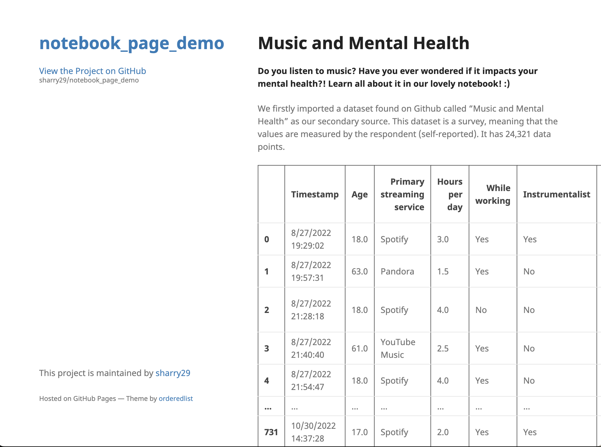
Hosting Your Project
We'll use GitHub Pages for this. You'll need to:
- Create a GitHub account
- Create a new repository on github.com and make sure that it's set to be public.
- Go to the settings of your repository by clicking the gear icon. Navigate to the "Pages" section in the list on the left.
- Enable GitHub Pages. Set the Source and Branch as follows.
Finally, independent of the option that you chose earlier, navigate back to the "Code" tab of your repository, press the "+" (Add File) button, select "Upload Files", and upload all of the files created by nbconvert. Then, after waiting a few minutes, you can see your "Deployments" in the bottom right. Click that link to find the URL for your page, which you can then preview. Tada! 🎉

To make any changes, simply edit the corresponding files in the GitHub editor. You can do that by opening the file and selecting the pencil icon for editing. There are also other themes you can try if you picked option 2 above.